Excel example 2 - STEM compatibility

Roche

2023-05-02

Introduction

This vignette describes how to work with the included example excel templates that are compatible to the survival models estimated with flexsurvPlus. These examples are deliberately simple and are intended to illustrate calculations in excel rather than as a basis for a real economic model. In this example the basic calculations needed to extrapolate survival are illustrated. This example is using the STEM bacward compatibility formulas.

Set up packages and data

Install packages

The following packages are required to run this example:

rm(list = ls())
# Libraries
library(flexsurvPlus)
library(tibble)
library(dplyr)
library(boot)
library(ggplot2)

Generate the data

To perform survival analyses, patient level data is required for the survival endpoints. In this example, we analyze progression-free survival (PFS). For more details on these steps please refer to the other vignettes.

# make reproducible
set.seed(1234)

# used later
(simulation_seed <- floor(runif(1, min = 1, max = 10^8)))
#> [1] 11370342
(bootstrap_seed <- floor(runif(1, min = 1, max = 10^8)))
#> [1] 62229940

# low number for speed of execution given illustrating concept
n_bootstrap <- 10

adtte <- sim_adtte(seed = simulation_seed)
head(adtte)
#>   USUBJID ARMCD             ARM PARAMCD                     PARAM AVAL AVALU
#> 1       1     A Reference Arm A     PFS Progression Free Survival  108  DAYS
#> 2       2     A Reference Arm A     PFS Progression Free Survival  150  DAYS
#> 3       3     A Reference Arm A     PFS Progression Free Survival  372  DAYS
#> 4       4     A Reference Arm A     PFS Progression Free Survival   73  DAYS
#> 5       5     A Reference Arm A     PFS Progression Free Survival  137  DAYS
#> 6       6     A Reference Arm A     PFS Progression Free Survival  103  DAYS
#>   CNSR
#> 1    0
#> 2    0
#> 3    0
#> 4    0
#> 5    0
#> 6    0

# subset PFS data and rename
PFS_data <- adtte %>%
  filter(PARAMCD == "PFS") %>%
  transmute(USUBJID,
    ARMCD,
    PFS_days = AVAL,
    PFS_event = 1 - CNSR
  )

Fitting the models

More information about each function can be used by running the code ?runPSM or viewing the other vignettes.

psm_PFS_all <- runPSM(
  data = PFS_data,
  time_var = "PFS_days",
  event_var = "PFS_event",
  model.type = c("Common shape"),
  distr = c(
    "exp",
    "weibull",
    "gompertz",
    "lnorm",
    "llogis",
    "gengamma",
    "gamma"
  ),
  strata_var = "ARMCD",
  int_name = "B",
  ref_name = "A"
)

Bootstrap the estimated parameters

As described in other vignettes we can use boot to explore uncertainty.

# fix seed for reproducible samples
set.seed(bootstrap_seed)

boot_psm_PFS_all <- do.call(boot, args = c(psm_PFS_all$config, statistic = bootPSM, R = n_bootstrap))

Converting to STEM format

As described in other vignettes we can use convSTEM function to transform the parameterisations for backwards compatibility to the SAS macro model formulas.

stemdata <- convSTEM(x = psm_PFS_all, samples = boot_psm_PFS_all, use = "complete.obs")

Exporting to Excel

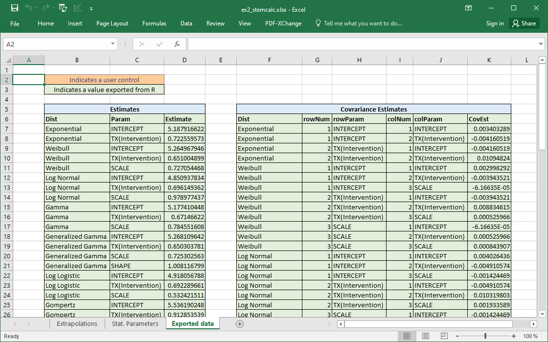
Once the values are calculated we can export to Excel. The following code prepares two tibbles that can be exported. One containing the main estimates. A second containing the covariance matrices.

main_estimates <- stemdata$stem_param %>%
  dplyr::transmute(Dist, Param, Estimate)

cov_estimates <- stemdata$stem_cov %>%
  dplyr::transmute(Dist, rowNum, rowParam, colNum, colParam, CovEst)

# can preview these tables

main_estimates %>%
  head() %>%
  pander::pandoc.table()
#> 
#> -------------------------------------------
#>     Dist            Param         Estimate 
#> ------------- ------------------ ----------
#>  Exponential      INTERCEPT        5.188   
#> 
#>  Exponential   TX(Intervention)    0.7226  
#> 
#>    Weibull        INTERCEPT        5.265   
#> 
#>    Weibull     TX(Intervention)    0.651   
#> 
#>    Weibull          SCALE          0.7271  
#> 
#>  Log Normal       INTERCEPT        4.851   
#> -------------------------------------------

cov_estimates %>%
  head() %>%
  pander::pandoc.table()
#> 
#> ---------------------------------------------------------------------------------
#>     Dist       rowNum       rowParam       colNum       colParam        CovEst   
#> ------------- -------- ------------------ -------- ------------------ -----------
#>  Exponential     1         INTERCEPT         1         INTERCEPT       0.003403  
#> 
#>  Exponential     1         INTERCEPT         2      TX(Intervention)   -0.004161 
#> 
#>  Exponential     2      TX(Intervention)     1         INTERCEPT       -0.004161 
#> 
#>  Exponential     2      TX(Intervention)     2      TX(Intervention)    0.01095  
#> 
#>    Weibull       1         INTERCEPT         1         INTERCEPT       0.002998  
#> 
#>    Weibull       1         INTERCEPT         2      TX(Intervention)   -0.003944 
#> ---------------------------------------------------------------------------------

# the following code is not run in the vignette but will export this file

# require(openxlsx)
# wb <- openxlsx::createWorkbook()
# openxlsx::addWorksheet(wb, sheetName = "Exported data")
# openxlsx::writeDataTable(wb, sheet = "Exported data", main_estimates, startRow = 2, startCol = 2)
# openxlsx::writeDataTable(wb, sheet = "Exported data", cov_estimates, startRow = 2, startCol = 3+ncol(main_estimates))
# openxlsx::saveWorkbook(wb, file = "export_data_ex2.xlsx", overwrite = TRUE)

The Excel model

Included with the package is an example Excel file called ex2_stemcalc.xlsx. This can be extracted using the below code (not run). It can also be found in the github repository at https://github.com/Roche/flexsurvPlus/tree/main/inst/extdata

installed_file <- system.file("extdata/ex2_stemcalc.xlsx", package = "flexsurvPlus")
installed_file
#> [1] "/usr/local/lib/R/site-library/flexsurvPlus/extdata/ex2_stemcalc.xlsx"

# not run but will give you a local copy of the file
# file.copy(from = installed_file, to ="copy_of_ex2_stemcalc.xlsx")

This illustrates how all the included survival models can be extrapolated in Excel.

Exported data tab

This contains a copy of the data exported in the last step.

Exported data tab

Stat. Parameters tab

This contains intermediary calculations needed when using the STEM parameterisation. This includes Cholesky decomposition of the calculated covariance matrix to implement PSA which are not needed when using the boot strap samples directly.

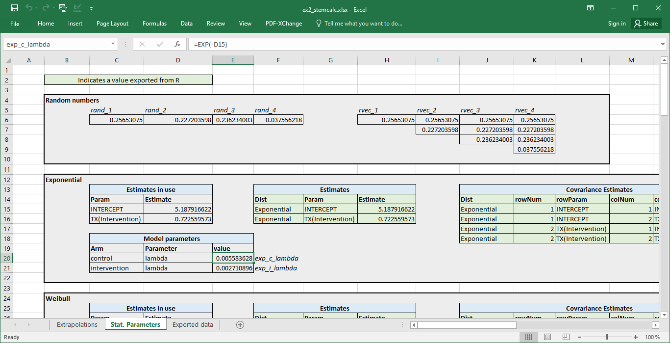
Stat. Parameters tab

Extrapolations tab

This contains example calculations to extrapolate survival.

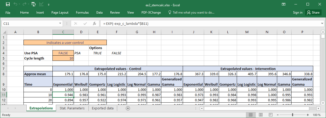
Extrapolations tab

We can compare the approximate estimates of mean survival with those calculated in R. As the excel model only goes until time t=2000 we can more directly compare to the estimates of restricted mean survival time (rmst) until this time.

means_est <- psm_PFS_all %>%
  summaryPSM(type = c("mean", "rmst"), t = 2000)

# match to selected model in screenshot
means_est %>%
  dplyr::filter(Model == "Common shape") %>%
  tidyr::pivot_wider(
    id_cols = c("Strata", "Dist"),
    names_from = c("type"),
    values_from = "value"
  ) %>%
  dplyr::arrange(Strata, Dist) %>%
  pander::pandoc.table()
#> 
#> --------------------------------------------------
#>     Strata            Dist          mean    rmst  
#> -------------- ------------------- ------- -------
#>  Intervention      Exponential      368.9   367.3 
#> 
#>  Intervention         Gamma         346.8   346.8 
#> 
#>  Intervention   Generalized Gamma   338.8   338.8 
#> 
#>  Intervention       Gompertz        326.3   326.3 
#> 
#>  Intervention     Log Logistic      459.4   405.7 
#> 
#>  Intervention      Log Normal       414.2   395.6 
#> 
#>  Intervention        Weibull         339     339  
#> 
#>   Reference        Exponential      179.1   179.1 
#> 
#>   Reference           Gamma         177.2   177.2 
#> 
#>   Reference     Generalized Gamma   176.8   176.8 
#> 
#>   Reference         Gompertz         175     175  
#> 
#>   Reference       Log Logistic      229.9   215.2 
#> 
#>   Reference        Log Normal       206.5   204.5 
#> 
#>   Reference          Weibull        176.8   176.8 
#> --------------------------------------------------