Excel example 3 - correlated endpoints in PSA
Roche
2023-05-02
Excel_example_ex3.RmdIntroduction
This vignette describes how to work with the included example excel templates that are compatible to the survival models estimated with flexsurvPlus. These examples are deliberately simple and are intended to illustrate calculations in excel rather than as a basis for a real economic model. In this example correlated endpoints are implemented in excel.
Set up packages and data
Generate the data
To perform survival analyses, patient level data is required for the survival endpoints. In this example, we analyze progression-free survival (PFS) and overall survival (OS). For more details on these steps please refer to the other vignettes.
# make reproducible
set.seed(1234)

# used later
(simulation_seed <- floor(runif(1, min = 1, max = 10^8)))
#> [1] 11370342
(bootstrap_seed <- floor(runif(1, min = 1, max = 10^8)))
#> [1] 62229940

# low number for speed of execution given illustrating concept
n_bootstrap <- 100

adtte <- sim_adtte(seed = simulation_seed, rho = 0.6)

# subset PFS data and rename
PFS_data <- adtte %>%
  filter(PARAMCD == "PFS") %>%
  transmute(USUBJID,
    ARMCD,
    PFS_days = AVAL,
    PFS_event = 1 - CNSR
  )

# subset PFS data and rename
OS_data <- adtte %>%
  filter(PARAMCD == "OS") %>%
  transmute(USUBJID,
    ARMCD,
    OS_days = AVAL,
    OS_event = 1 - CNSR
  )

OSPFS_data <- PFS_data %>%
  left_join(OS_data, by = c("USUBJID", "ARMCD"))

head(OSPFS_data)
#>   USUBJID ARMCD PFS_days PFS_event OS_days OS_event
#> 1       1     A      185         1     600        0
#> 2       2     A      149         1     618        0
#> 3       3     A      418         1     525        0
#> 4       4     A       80         1     492        0
#> 5       5     A      345         1     595        0
#> 6       6     A      118         1     537        0
Fitting the models
More information about each function can be used by running the code ?runPSM or viewing the other vignettes. Here only common shape models are fit but the same concept applies to all other models.
psm_PFS_all <- runPSM(
  data = OSPFS_data,
  time_var = "PFS_days",
  event_var = "PFS_event",
  model.type = c("Common shape"),
  distr = c(
    "exp",
    "weibull",
    "gompertz",
    "lnorm",
    "llogis",
    "gengamma",
    "gamma",
    "genf"
  ),
  strata_var = "ARMCD",
  int_name = "B",
  ref_name = "A"
)


psm_OS_all <- runPSM(
  data = OSPFS_data,
  time_var = "OS_days",
  event_var = "OS_event",
  model.type = c("Common shape"),
  distr = c(
    "exp",
    "weibull",
    "gompertz",
    "lnorm",
    "llogis",
    "gengamma",
    "gamma",
    "genf"
  ),
  strata_var = "ARMCD",
  int_name = "B",
  ref_name = "A"
)
Bootstrap the estimated parameters
As described in other vignettes we can use boot to
explore uncertainty. We can also reuse the seed to maintain correlations
by ensuring the same individuals are sampled across each endpoint
# fix seed for reproducible samples
set.seed(bootstrap_seed)

boot_psm_PFS_all <- do.call(boot, args = c(psm_PFS_all$config, statistic = bootPSM, R = n_bootstrap))

# reuse the seed to maintain correlations
set.seed(bootstrap_seed)

boot_psm_OS_all <- do.call(boot, args = c(psm_OS_all$config, statistic = bootPSM, R = n_bootstrap))
Exporting to Excel
Once the values are calculated we can export to Excel. The following code prepares four tibbles that can be exported. Two containing the main estimates for PFS & OS respectively. And two more containing the bootstrap samples.
main_estimates_PFS <- psm_PFS_all$parameters_vector %>%
  t() %>%
  as.data.frame()

main_estimates_OS <- psm_OS_all$parameters_vector %>%
  t() %>%
  as.data.frame()

boot_estimates_PFS <- boot_psm_PFS_all$t %>%
  as.data.frame()

boot_estimates_OS <- boot_psm_OS_all$t %>%
  as.data.frame()

colnames(main_estimates_PFS) <- colnames(boot_estimates_PFS) <- names(psm_PFS_all$parameters_vector)

colnames(main_estimates_OS) <- colnames(boot_estimates_OS) <- names(psm_OS_all$parameters_vector)

# can preview these tables

main_estimates_PFS[, 1:5] %>%
  pander::pandoc.table()
#>
#> ----------------------------------------------------------------
#>  comshp.exp.rate.int   comshp.exp.rate.ref   comshp.exp.rate.TE
#> --------------------- --------------------- --------------------
#>       0.002327              0.004945               -0.754
#> ----------------------------------------------------------------
#>
#> Table: Table continues below
#>
#>
#> -----------------------------------------------------
#>  comshp.weibull.scale.int   comshp.weibull.scale.ref
#> -------------------------- --------------------------
#>           421.4                      216.1
#> -----------------------------------------------------

# the following code is not run in the vignette but will export this file

# require(openxlsx)
# wb <- openxlsx::createWorkbook()
# openxlsx::addWorksheet(wb, sheetName = "PFS Exported data")
# openxlsx::writeDataTable(wb, sheet = "PFS Exported data", main_estimates_PFS, startRow = 2, startCol = 3)
# openxlsx::writeDataTable(wb, sheet = "PFS Exported data", boot_estimates_PFS, startRow = 5, startCol = 2, rowNames = TRUE)
# openxlsx::createNamedRegion(wb, sheet = "PFS Exported data",
#                             cols = 2:(2+length(main_estimates_PFS)), rows = 3, name = "PFS_Estimates")
# openxlsx::createNamedRegion(wb, sheet = "PFS Exported data",
#                             cols = 2:(2+length(main_estimates_PFS)), rows = 6:(6-1+nrow(boot_estimates_PFS)), name = "PFS_Samples")
# openxlsx::addWorksheet(wb, sheetName = "OS Exported data")
# openxlsx::writeDataTable(wb, sheet = "OS Exported data", main_estimates_OS, startRow = 2, startCol = 3)
# openxlsx::writeDataTable(wb, sheet = "OS Exported data", boot_estimates_OS, startRow = 5, startCol = 2, rowNames = TRUE)
# openxlsx::createNamedRegion(wb, sheet = "OS Exported data",
#                             cols = 2:(2+length(main_estimates_OS)), rows = 3, name = "OS_Estimates")
# openxlsx::createNamedRegion(wb, sheet = "OS Exported data",
#                             cols = 2:(2+length(main_estimates_OS)), rows = 6:(6-1+nrow(boot_estimates_OS)), name = "OS_Samples")
# openxlsx::saveWorkbook(wb, file = "export_data.xlsx", overwrite = TRUE)
The Excel model
Included with the package is an example Excel file called
ex3_correlation.xlsm. This can be extracted using the below
code (not run). It can also be found in the github repository at https://github.com/Roche/flexsurvPlus/tree/main/inst/extdata.
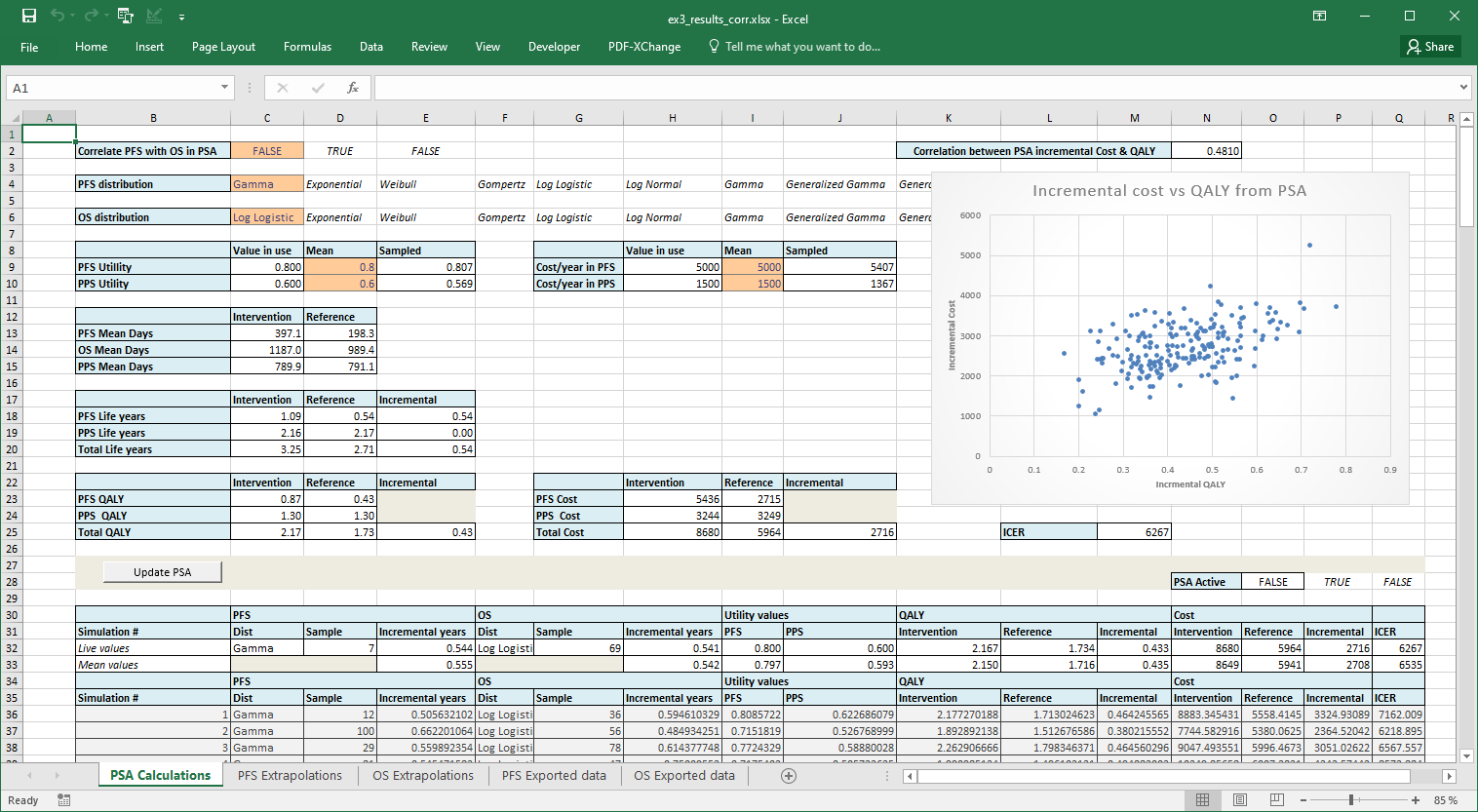
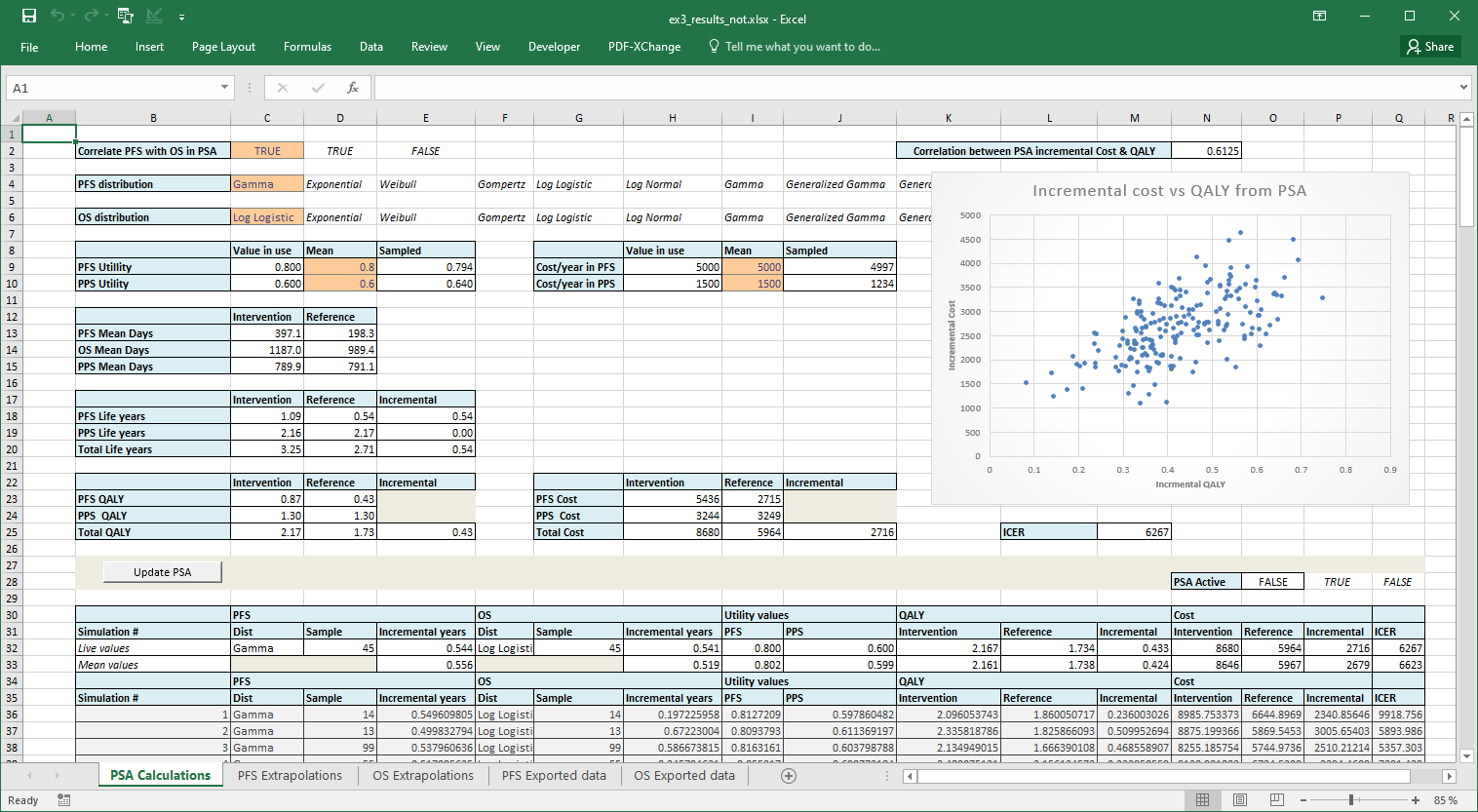
Also included are two files with pre calculated results for correlated
and un-correlated PSA and excluding the excel PSA macro. These are
ex3_results_corr.xlsx for correlated PSA and
ex3_results_not.xlsx for un-correlated.
installed_file <- system.file("extdata/ex3_correlation.xlsm", package = "flexsurvPlus")
installed_file
#> [1] "/usr/local/lib/R/site-library/flexsurvPlus/extdata/ex3_correlation.xlsm"

# not run but will give you a local copy of the file
# file.copy(from = installed_file, to ="ex3_correlation.xlsm")
This illustrates how all the included survival models can be extrapolated in Excel and PSA setup to correlate two outcomes.