Introduction

This vignette provides a short example of a Bayesian NMA for HR data. The model fit relies on the gemtc package, pre- and post-processing is done with gemtcPlus.

Prepare the environment

knitr::opts_chunk$set(echo = TRUE)

library(dplyr)
library(gemtc)
library(gemtcPlus)
library(ggmcmc)

Load in the data

# load example data
data("hr_data", package = "gemtcPlus")

Plan the model

#Plan model
model_plan <- plan_hr(bth.model = "FE", 
                          n.chain = 3, 
                          n.iter = 6000, 
                          thin = 1,
                          n.adapt = 1000, 
                          link = "identity",
                          linearModel = "fixed")

Ready the data

model_input <-  nma_pre_proc(data = hr_data, plan = model_plan)

Fit the model

model  <- nma_fit(model_input = model_input)

## Warning in (function (network, type = "consistency", factor = 2.5, n.chain =
## 4, : Likelihood can not be inferred. Defaulting to normal.

## Compiling model graph
##    Resolving undeclared variables
##    Allocating nodes
## Graph information:
##    Observed stochastic nodes: 7
##    Unobserved stochastic nodes: 5
##    Total graph size: 132
## 
## Initializing model

Post processing

ggs_traceplot(ggs(model$samples))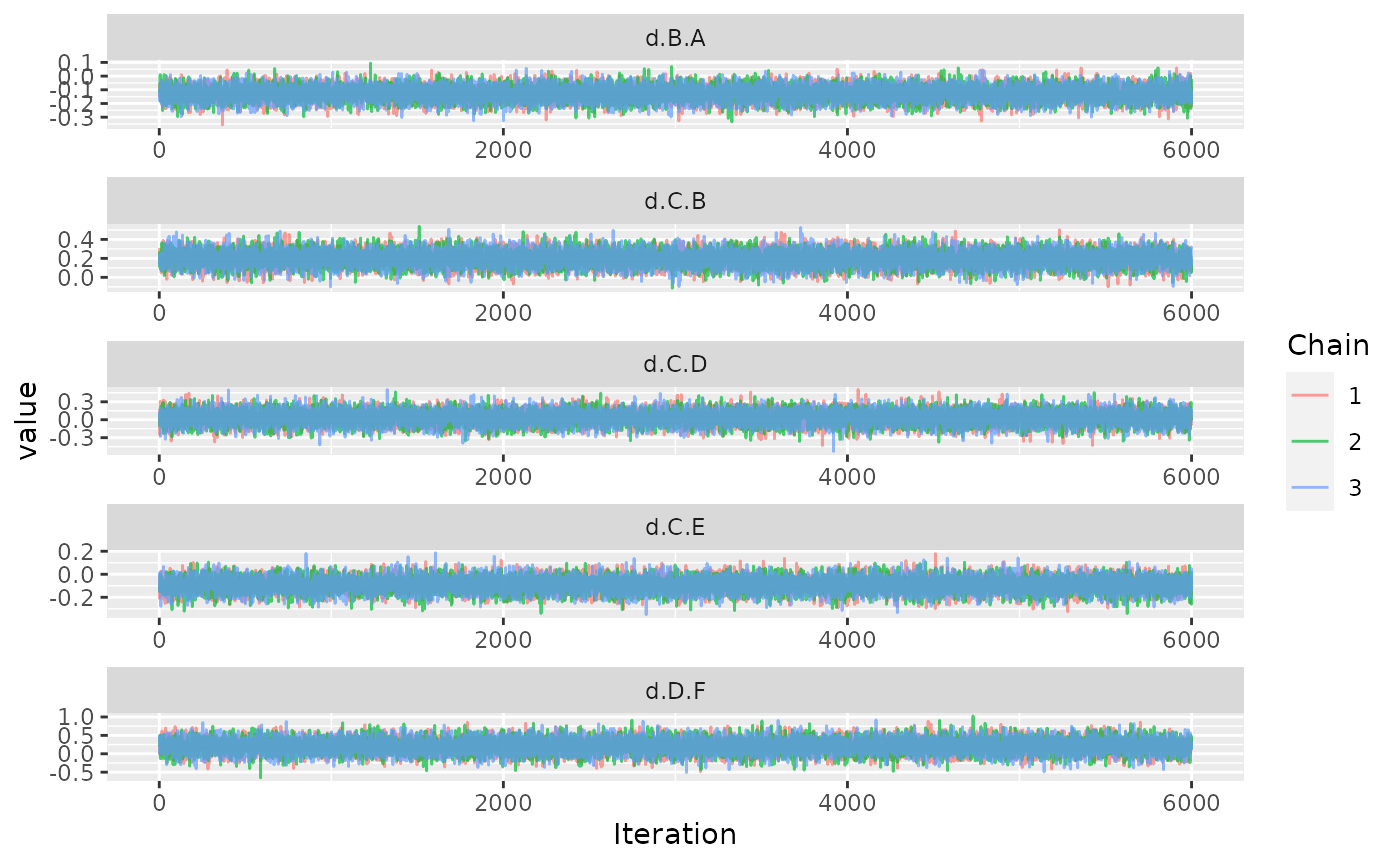

ggs_density(ggs(model$samples))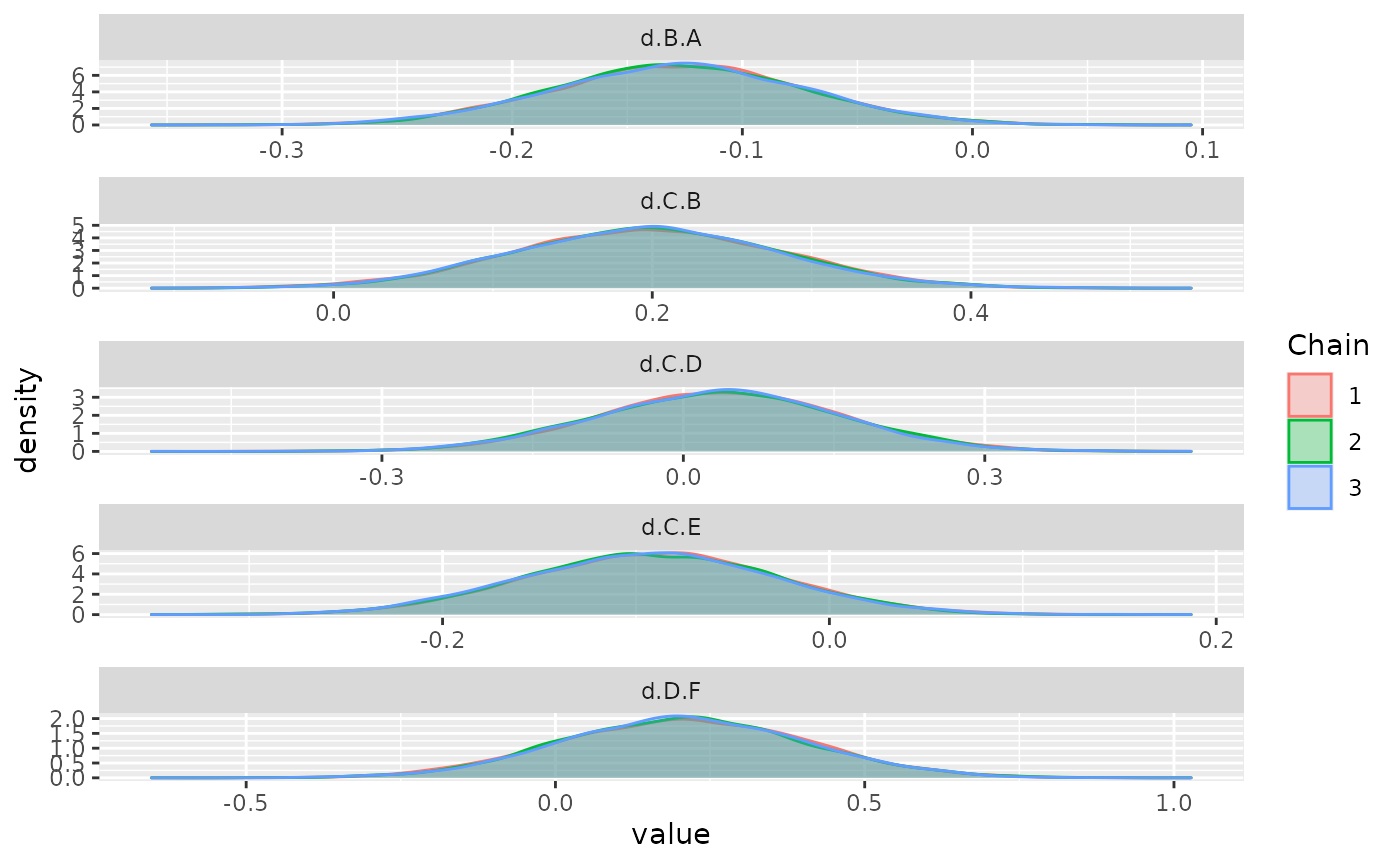

summary(model)

## 
## Results on the Mean Difference scale
## 
## Iterations = 1:6000
## Thinning interval = 1 
## Number of chains = 3 
## Sample size per chain = 6000 
## 
## 1. Empirical mean and standard deviation for each variable,
##    plus standard error of the mean:
## 
##           Mean      SD  Naive SE Time-series SE
## d.B.A -0.12792 0.05541 0.0004130      0.0004044
## d.C.B  0.19765 0.08313 0.0006196      0.0006196
## d.C.D  0.03549 0.12051 0.0008983      0.0009557
## d.C.E -0.09321 0.06649 0.0004956      0.0005243
## d.D.F  0.20852 0.19508 0.0014540      0.0014541
## 
## 2. Quantiles for each variable:
## 
##           2.5%      25%      50%      75%    97.5%
## d.B.A -0.23611 -0.16600 -0.12790 -0.09026 -0.01820
## d.C.B  0.03457  0.14126  0.19849  0.25451  0.35855
## d.C.D -0.20200 -0.04492  0.03748  0.11554  0.26981
## d.C.E -0.22370 -0.13805 -0.09306 -0.04824  0.03684
## d.D.F -0.17147  0.07815  0.20894  0.33972  0.59366
## 
## -- Model fit (residual deviance):
## 
##      Dbar        pD       DIC 
##  5.479850  4.978586 10.458436 
## 
## 7 data points, ratio 0.7828, I^2 = 0%

plot(model_input$fitting_data)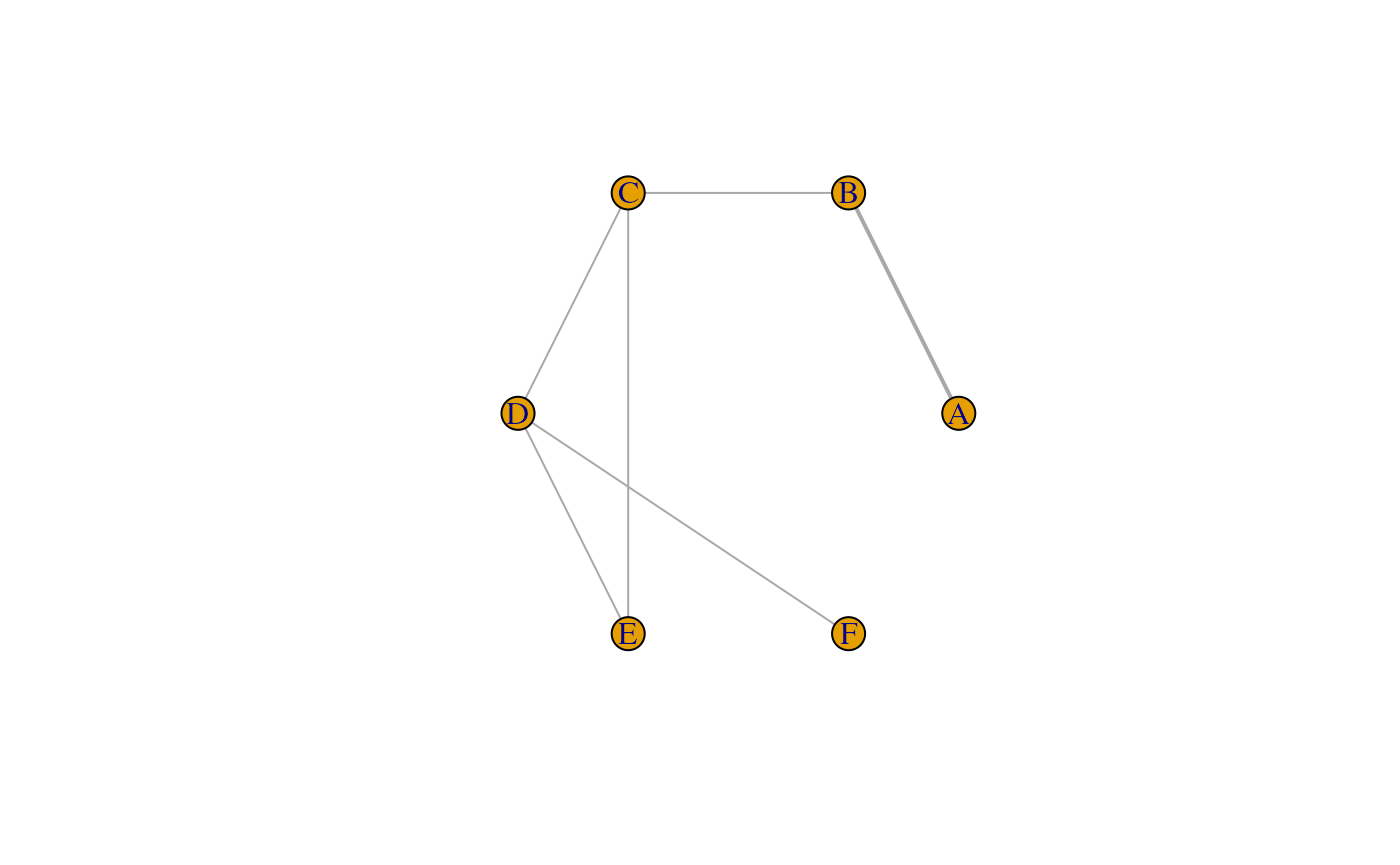

get_mtc_sum(model)

##     DIC   pD resDev dataPoints
## 1 10.46 4.98   5.48          7

Random Effects example

Update model plan and re-run fit.

#Plan model
model_plan <- plan_hr(bth.model = "RE", 
                      n.chain = 3,
                      n.iter = 6000,
                      thin = 1,
                      n.adapt = 1000,
                      link = "identity",
                      linearModel = "random", 
                      bth.prior = mtc.hy.prior(type = "var", distr = "dlnorm",-4.18, 1 / 1.41 ^ 2)
)

Fit the model

model  <- nma_fit(model_input = model_input)

## Warning in (function (network, type = "consistency", factor = 2.5, n.chain =
## 4, : Likelihood can not be inferred. Defaulting to normal.

## Compiling model graph
##    Resolving undeclared variables
##    Allocating nodes
## Graph information:
##    Observed stochastic nodes: 7
##    Unobserved stochastic nodes: 5
##    Total graph size: 132
## 
## Initializing model

Post processing

Inspect convergence

The ggmcmc package provides ggplot2 versions of all major convergence plots and diagnostics.

Figure Traceplot

ggs_traceplot(ggs(model$samples))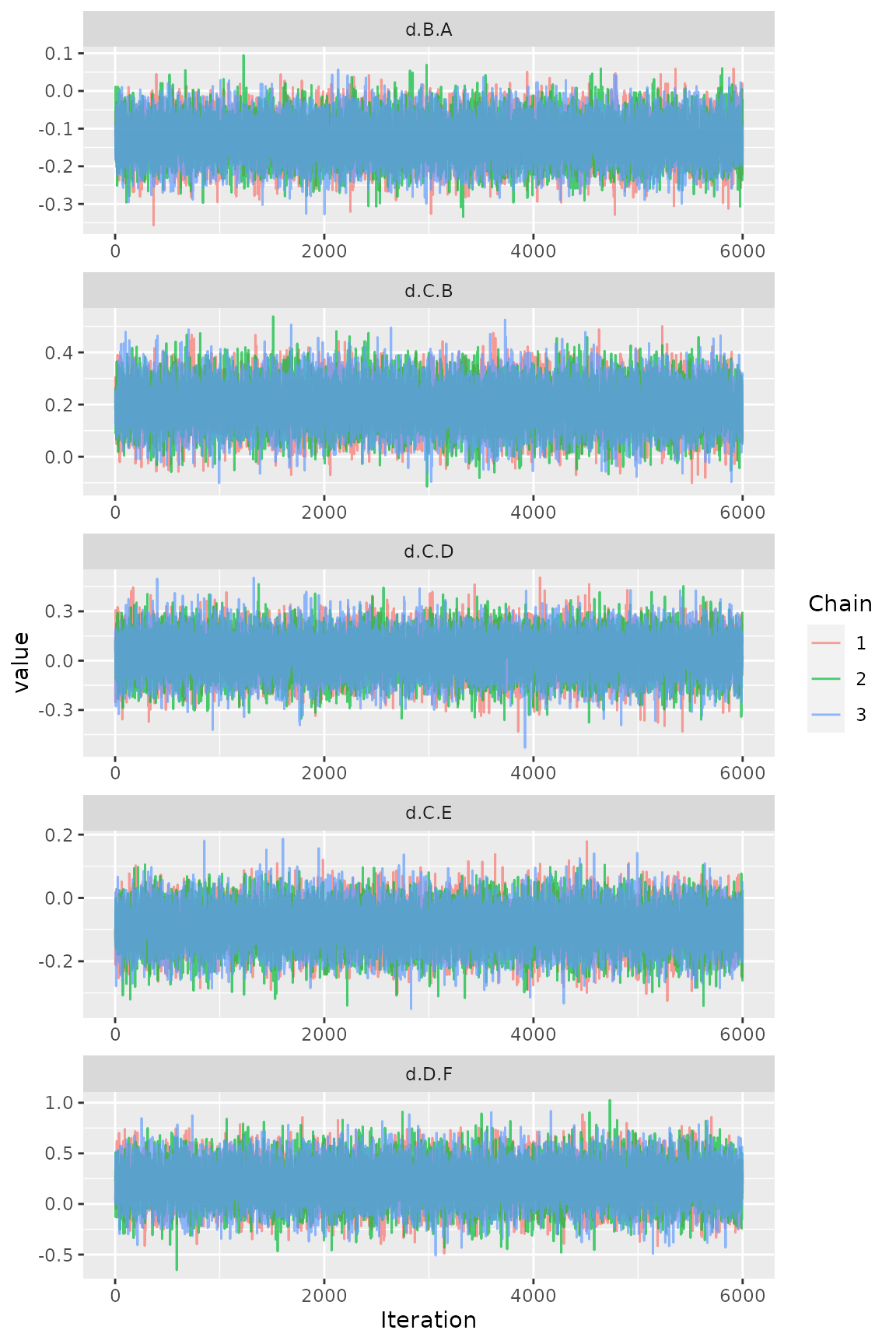

Figure Densityplot

ggs_density(ggs(model$samples))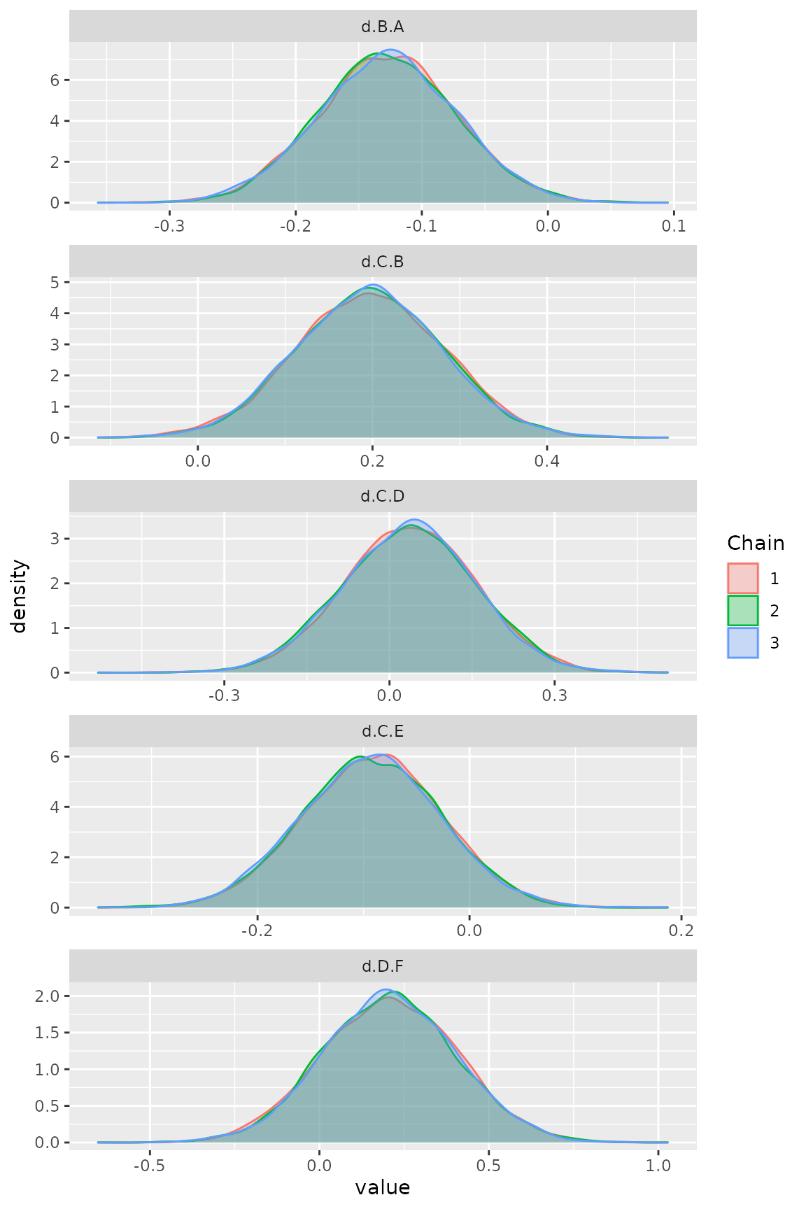

Figure Brooks-Gelman-Rubin convergence diagnostic (Rhat)

ggs_Rhat(ggs(model$samples))

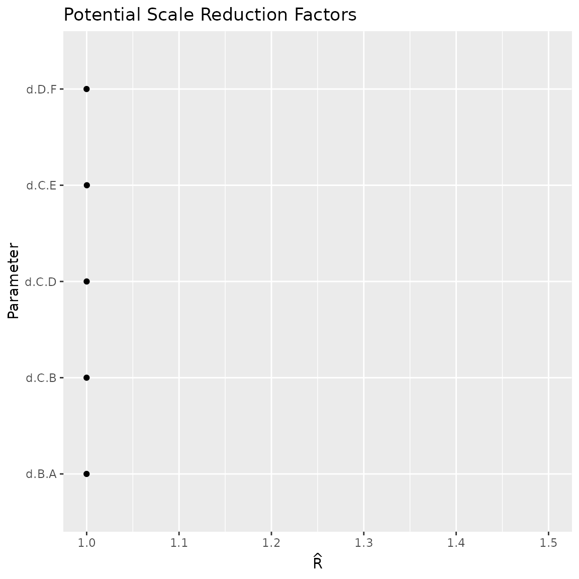
Figure Auto-correlation plot

ggs_autocorrelation(ggs(model$samples))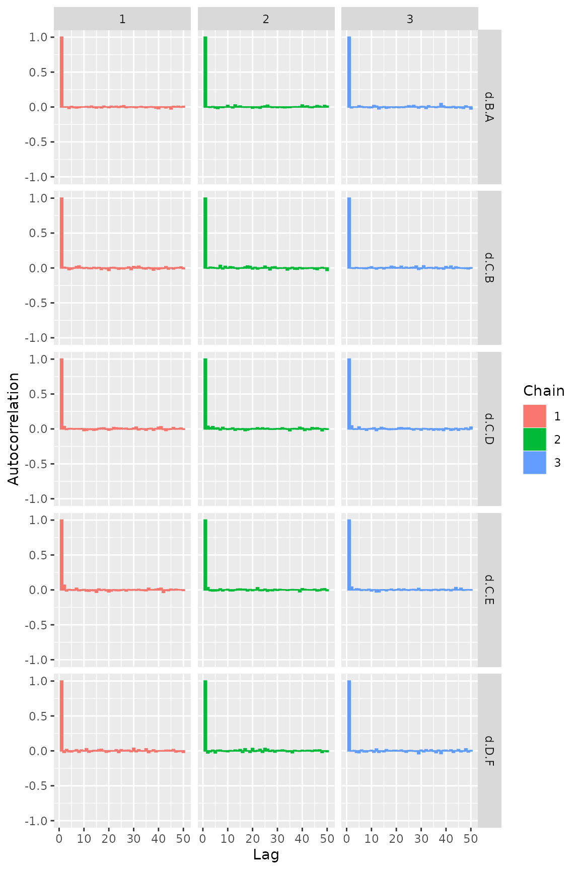

Figure Running means

ggs_running(ggs(model$samples))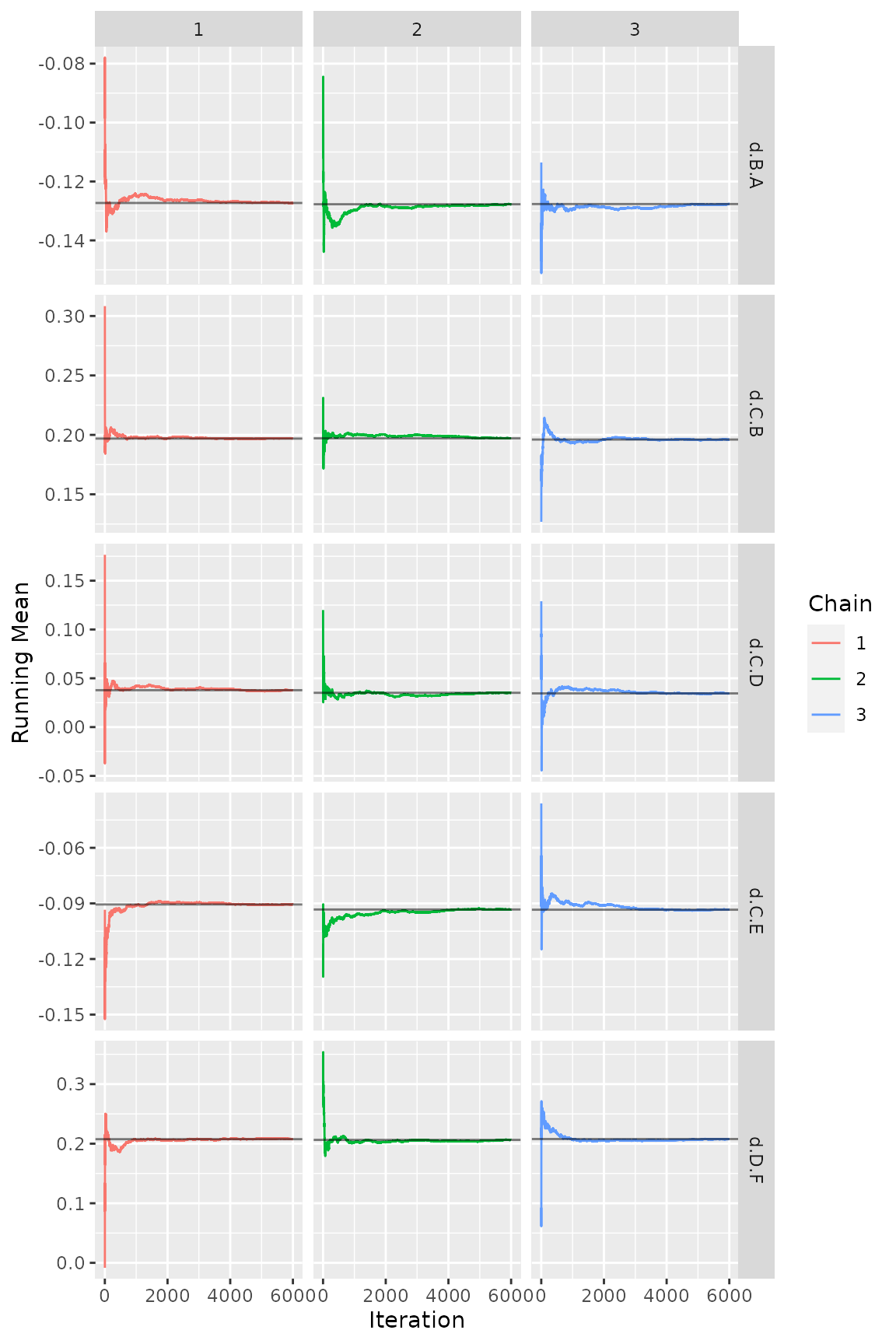

Produce outputs of interest

Posterior summaries (log-scale)

The contrasts in this model are log-hazard ratios (which correspond to differences in log-hazard rates).

Unfortunately, gemtc does not provide an estimate of the effective sample size (n.eff). Instead, a time-series SE is given. As a rule of thumb, the length of the MCMC is sufficient if the time-series SE is smaller than 2%(-5%) of the posterior SD.

summary(model)

## 
## Results on the Mean Difference scale
## 
## Iterations = 1:6000
## Thinning interval = 1 
## Number of chains = 3 
## Sample size per chain = 6000 
## 
## 1. Empirical mean and standard deviation for each variable,
##    plus standard error of the mean:
## 
##           Mean      SD  Naive SE Time-series SE
## d.B.A -0.12792 0.05541 0.0004130      0.0004044
## d.C.B  0.19765 0.08313 0.0006196      0.0006196
## d.C.D  0.03549 0.12051 0.0008983      0.0009557
## d.C.E -0.09321 0.06649 0.0004956      0.0005243
## d.D.F  0.20852 0.19508 0.0014540      0.0014541
## 
## 2. Quantiles for each variable:
## 
##           2.5%      25%      50%      75%    97.5%
## d.B.A -0.23611 -0.16600 -0.12790 -0.09026 -0.01820
## d.C.B  0.03457  0.14126  0.19849  0.25451  0.35855
## d.C.D -0.20200 -0.04492  0.03748  0.11554  0.26981
## d.C.E -0.22370 -0.13805 -0.09306 -0.04824  0.03684
## d.D.F -0.17147  0.07815  0.20894  0.33972  0.59366
## 
## -- Model fit (residual deviance):
## 
##      Dbar        pD       DIC 
##  5.479850  4.978586 10.458436 
## 
## 7 data points, ratio 0.7828, I^2 = 0%

In the example here, the chain length seems borderline (sufficient for posterior means and medians, but rather a bit too small for stable 95% credible intervals).

To judge overall model fit, the residual deviance should be compared to the number of independent data points (which can be done via a small utility function in gemtcPlus).

get_mtc_sum(model)

##     DIC   pD resDev dataPoints
## 1 10.46 4.98   5.48          7

Hazard ratio estimates

Assume new treatment is “A” and is to be compared vs all other treatments.

Table Hazard ratios A vs other treatments

HR <- get_mtc_newVsAll(model, new.lab = "A", transform = "exp", digits = 2)
HR

##   Comparator  Med CIlo CIup
## 1          B 0.88 0.79 0.98
## 2          C 1.07 0.88 1.30
## 3          D 1.03 0.76 1.41
## 4          E 1.18 0.93 1.49
## 5          F 0.84 0.51 1.38

Table Probability A better than other treatments (better meaning smaller HR)

get_mtc_probBetter(model, new.lab = "A", smaller.is.better = TRUE, sort.by = "effect")

##   New Comparator probNewBetter
## 1   A          B         0.990
## 5   A          F         0.757
## 3   A          D         0.415
## 2   A          C         0.245
## 4   A          E         0.091

Figure Forest plot A vs other treatments

plot_mtc_forest(x = HR, lab = "Hazard ratio A vs others", sort.by = "effect")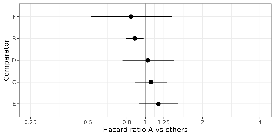

Table Cross-tabulation of HRs

ctab <- round(exp(relative.effect.table(model)), 2)
pander::pandoc.table(as.data.frame(ctab), split.tables = Inf)

	A	B	C	D	E	F
A	A	1.14 (1.02, 1.27)	0.93 (0.77, 1.13)	0.97 (0.71, 1.31)	0.85 (0.67, 1.08)	1.19 (0.72, 1.95)
B	0.88 (0.79, 0.98)	B	0.82 (0.7, 0.97)	0.85 (0.64, 1.13)	0.75 (0.61, 0.92)	1.05 (0.65, 1.69)
C	1.07 (0.88, 1.3)	1.22 (1.04, 1.43)	C	1.04 (0.82, 1.31)	0.91 (0.8, 1.04)	1.28 (0.81, 1.99)
D	1.03 (0.76, 1.41)	1.18 (0.88, 1.57)	0.96 (0.76, 1.22)	D	0.88 (0.69, 1.12)	1.23 (0.84, 1.81)
E	1.18 (0.93, 1.49)	1.34 (1.08, 1.65)	1.1 (0.96, 1.25)	1.14 (0.89, 1.45)	E	1.4 (0.89, 2.21)
F	0.84 (0.51, 1.38)	0.95 (0.59, 1.55)	0.78 (0.5, 1.23)	0.81 (0.55, 1.19)	0.71 (0.45, 1.12)	F

Treatment rankings

rk  <- rank.probability(model, preferredDirection = -1)
mrk <- reshape2::melt(rk[,], varnames = c("Treatment", "Rank"), value.name = "Probability")

fig <- ggplot(data = mrk) +
  geom_line(aes(Rank, Probability, color = Treatment, linetype = Treatment), size = 1.5) +
  theme_bw()

## Warning: Using `size` aesthetic for lines was deprecated in ggplot2 3.4.0.
## ℹ Please use `linewidth` instead.
## This warning is displayed once every 8 hours.
## Call `lifecycle::last_lifecycle_warnings()` to see where this warning was
## generated.

Figure Rankogram

plot(fig)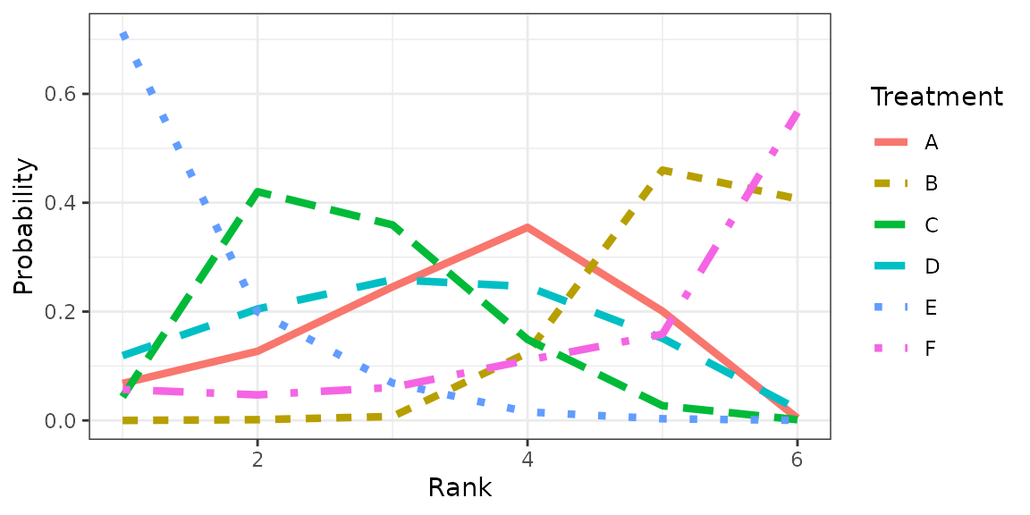

Table Rank probabilities

colnames(rk) <- paste("Rank", 1:ncol(rk))
rk

## Rank probability; preferred direction = -1
##       Rank 1      Rank 2     Rank 3     Rank 4      Rank 5       Rank 6
## A 0.06977778 0.127111111 0.24400000 0.35405556 0.200277778 0.0047777778
## B 0.00000000 0.001666667 0.00650000 0.12511111 0.459388889 0.4073333333
## C 0.04305556 0.419722222 0.36127778 0.14927778 0.025888889 0.0007777778
## D 0.11794444 0.205166667 0.26027778 0.24566667 0.151666667 0.0192777778
## E 0.71277778 0.200333333 0.06811111 0.01594444 0.002555556 0.0002777778
## F 0.05644444 0.046000000 0.05983333 0.10994444 0.160222222 0.5675555556

Extract model code (e.g. for Appendix)

cat(model$model$code)

## model {
##  # Likelihood for arm-based data
##  ## OMITTED
##  # Likelihood for contrast-based data (univariate for 2-arm trials)
##  for(i in studies.r2) {
##      for (k in 2:na[i]) {
##          mest[i, k] <- delta[i, k]
##      }
##      m[i, 2] ~ dnorm(mest[i, 2], prec[i, 2])
##      prec[i, 2] <- 1 / (e[i, 2] * e[i, 2])
##  
##      dev[i, 1] <- pow(m[i, 2] - mest[i, 2], 2) * prec[i, 2]
##  }
##  # Likelihood for contrast-based data (multivariate for multi-arm trials)
##  ## OMITTED
## 
##  # Fixed effect model
##  for (i in studies) {
##      delta[i, 1] <- 0
##      for (k in 2:na[i]) {
##          delta[i, k] <- d[t[i, 1], t[i, k]]
##      }
##  }
## 
##  # Relative effect matrix
##  d[1, 1] <- 0
##  d[1, 2] <- -d.B.A
##  d[1, 3] <- -d.B.A + -d.C.B
##  d[1, 4] <- -d.B.A + -d.C.B + d.C.D
##  d[1, 5] <- -d.B.A + -d.C.B + d.C.E
##  d[1, 6] <- -d.B.A + -d.C.B + d.C.D + d.D.F
##  for (i in 2:nt) {
##      for (j in 1:nt) {
##          d[i, j] <- d[1, j] - d[1, i]
##      }
##  }
## 
##  prior.prec <- pow(re.prior.sd, -2)
## 
##  # Study baseline priors
##  ## OMITTED
## 
##  # Effect parameter priors
##  d.B.A ~ dnorm(0, prior.prec)
##  d.C.B ~ dnorm(0, prior.prec)
##  d.C.D ~ dnorm(0, prior.prec)
##  d.C.E ~ dnorm(0, prior.prec)
##  d.D.F ~ dnorm(0, prior.prec)
##  
## }

Session info

BEE repository: C:/Users/seom1/Documents/GitHub/gemtcPlus/vignettes

date()

## [1] "Thu Apr 24 15:46:41 2025"

sessionInfo()

## R version 4.2.2 (2022-10-31 ucrt)
## Platform: x86_64-w64-mingw32/x64 (64-bit)
## Running under: Windows 10 x64 (build 22631)
## 
## Matrix products: default
## 
## locale:
## [1] LC_COLLATE=German_Switzerland.utf8  LC_CTYPE=German_Switzerland.utf8   
## [3] LC_MONETARY=German_Switzerland.utf8 LC_NUMERIC=C                       
## [5] LC_TIME=German_Switzerland.utf8    
## 
## attached base packages:
## [1] stats     graphics  grDevices utils     datasets  methods   base     
## 
## other attached packages:
## [1] ggmcmc_1.5.1.1  ggplot2_3.4.1   tidyr_1.3.0     gemtcPlus_1.0.0
## [5] R2jags_0.7-1    rjags_4-14      gemtc_1.0-1     coda_0.19-4    
## [9] dplyr_1.1.4    
## 
## loaded via a namespace (and not attached):
##  [1] sass_0.4.4           jsonlite_1.8.4       splines_4.2.2       
##  [4] network_1.18.1       bslib_0.4.2          highr_0.10          
##  [7] metafor_4.0-0        pander_0.6.5         yaml_2.3.6          
## [10] R2WinBUGS_2.1-21     numDeriv_2016.8-1.1  pillar_1.9.0        
## [13] lattice_0.20-45      glue_1.6.2           digest_0.6.31       
## [16] RColorBrewer_1.1-3   meta_6.2-1           minqa_1.2.5         
## [19] colorspace_2.1-0     htmltools_0.5.4      Matrix_1.5-1        
## [22] plyr_1.8.8           pkgconfig_2.0.3      purrr_1.0.1         
## [25] scales_1.2.1         metadat_1.2-0        lme4_1.1-32         
## [28] tibble_3.2.1         farver_2.1.1         generics_0.1.3      
## [31] cachem_1.0.6         withr_2.5.0          cli_3.6.0           
## [34] crayon_1.5.2         magrittr_2.0.3       statnet.common_4.8.0
## [37] memoise_2.0.1        evaluate_0.20        GGally_2.1.2        
## [40] fs_1.6.1             fansi_1.0.4          nlme_3.1-160        
## [43] MASS_7.3-58.1        forcats_1.0.0        xml2_1.3.3          
## [46] truncnorm_1.0-9      textshaping_0.3.6    tools_4.2.2         
## [49] lifecycle_1.0.3      stringr_1.5.0        munsell_0.5.0       
## [52] compiler_4.2.2       pkgdown_1.6.1        jquerylib_0.1.4     
## [55] systemfonts_1.0.4    rlang_1.1.3          grid_4.2.2          
## [58] nloptr_2.0.3         rstudioapi_0.14      CompQuadForm_1.4.3  
## [61] igraph_1.4.2         labeling_0.4.2       rmarkdown_2.20      
## [64] boot_1.3-28          gtable_0.3.1         abind_1.4-5         
## [67] reshape_0.8.9        reshape2_1.4.4       R6_2.5.1            
## [70] knitr_1.41           fastmap_1.1.0        utf8_1.2.3          
## [73] mathjaxr_1.6-0       rprojroot_2.0.3      ragg_1.2.5          
## [76] desc_1.4.2           stringi_1.7.12       parallel_4.2.2      
## [79] Rcpp_1.0.10          vctrs_0.6.5          tidyselect_1.2.0    
## [82] xfun_0.36

Bayesian FE & RE NMA for HR data (via gemtc package) - Result Generation

Sandro Gsteiger, Nick Howlett

2025-04-24

Introduction

Prepare the environment

Load in the data

Plan the model

Ready the data

Fit the model

Post processing

Random Effects example

Fit the model

Post processing

Inspect convergence

Produce outputs of interest

Posterior summaries (log-scale)

Hazard ratio estimates

Treatment rankings

Extract model code (e.g. for Appendix)

Session info