Bootstrapping for MAIC weighted hazard ratios
bootstrap_HR.RdBootstrapping for MAIC weighted hazard ratios
bootstrap_HR(
  intervention_data,
  matching,
  i,
  model,
  comparator_data,
  min_weight = 1e-04
)
Arguments
- intervention_data
A data frame containing individual patient data from the intervention study.
- matching
A character vector giving the names of the covariates to use in matching. These names must match the column names in intervention_data.
- i
Index used to select a sample within
boot.- model
A model formula in the form 'Surv(Time, Event==1) ~ ARM'. Variable names need to match the corresponding columns in intervention_data.
- comparator_data
A data frame containing pseudo individual patient data from the comparator study needed to derive the relative treatment effect. The outcome variables names must match intervention_data.
- min_weight
A numeric value that defines the minimum weight allowed. This value (default 0.0001) will replace weights estimated at 0 in a sample.
Value
The HR as a numeric value.
Details
This function is intended to be used in conjunction with the
boot function to return the statistic to be
bootstrapped. In this case by performing MAIC weighting using
estimate_weights and returning a weighted hazard ratio (HR) from a
Cox proportional hazards model. This is used as the 'statistic' argument in
the boot function.
See also
Examples
# This example code combines weighted individual patient data for 'intervention'
# and pseudo individual patient data for 'comparator' and performs analyses for
# two endpoints: overall survival (a time to event outcome) and objective
# response (a binary outcome)
library(dplyr)
#>
#> Attaching package: ‘dplyr’
#> The following objects are masked from ‘package:stats’:
#>
#> filter, lag
#> The following objects are masked from ‘package:base’:
#>
#> intersect, setdiff, setequal, union
library(boot)
library(survival)
#>
#> Attaching package: ‘survival’
#> The following object is masked from ‘package:boot’:
#>
#> aml
library(MAIC)
library(ggplot2)
library(survminer)
#> Loading required package: ggpubr
library(flextable)
#>
#> Attaching package: ‘flextable’
#> The following objects are masked from ‘package:ggpubr’:
#>
#> border, font, rotate
library(officer)
# load intervention data with weights saved in est_weights
data(est_weights, package = "MAIC")
# Combine data -----------------------------------------------------------------
# Combine the the comparator pseudo data with the analysis data, outputted from
# the estimate_weights function
# Read in digitised pseudo survival data for the comparator
comparator_surv <- read.csv(system.file("extdata", "psuedo_IPD.csv",
package = "MAIC", mustWork = TRUE)) %>%
rename(Time=Time, Event=Event)
# Simulate response data based on the known proportion of responders
comparator_n <- nrow(comparator_surv) # total number of patients in the comparator data
comparator_prop_events <- 0.4 # proportion of responders
# Calculate number with event
# Use round() to ensure we end up with a whole number of people
# number without an event = Total N - number with event to ensure we keep the
# same number of patients
n_with_event <- round(comparator_n*comparator_prop_events, digits = 0)
comparator_binary <- data.frame("response"= c(rep(1, n_with_event), rep(0, comparator_n - n_with_event)))
# Join survival and response comparator data
# Note the rows do not represent observations from a particular patient
# i.e. there is no relationship between the survival time and response status
# for a given row since this is simulated data
# In a real data set this relationship would be present
comparator_input <- cbind(comparator_surv, comparator_binary) %>%
mutate(wt=1, wt_rs=1, ARM="Comparator") # All patients have weight = 1
head(comparator_input)
#> Time Event response wt wt_rs ARM
#> 1 20.2311676 1 1 1 1 Comparator
#> 2 28.7679537 1 1 1 1 Comparator
#> 3 41.0662129 0 1 1 1 Comparator
#> 4 0.8492261 1 1 1 1 Comparator
#> 5 9.0521882 0 1 1 1 Comparator
#> 6 3.4450075 1 1 1 1 Comparator
# Join comparator data with the intervention data (naming of variables should be
# consistent between both datasets)
# Set factor levels to ensure "Comparator" is the reference treatment
combined_data <- bind_rows(est_weights$analysis_data, comparator_input)
combined_data$ARM <- relevel(as.factor(combined_data$ARM), ref="Comparator")
#### Estimating the relative effect --------------------------------------------
### Example for survival data --------------------------------------------------
## Kaplan-Meier plot
# Unweighted intervention data
KM_int <- survfit(formula = Surv(Time, Event==1) ~ 1 ,
data = est_weights$analysis_data,
type="kaplan-meier")
# Weighted intervention data
KM_int_wtd <- survfit(formula = Surv(Time, Event==1) ~ 1 ,
data = est_weights$analysis_data,
weights = wt,
type="kaplan-meier")
# Comparator data
KM_comp <- survfit(formula = Surv(Time, Event==1) ~ 1 ,
data = comparator_input,
type="kaplan-meier")
# Combine the survfit objects ready for ggsurvplot
KM_list <- list(Intervention = KM_int,
Intervention_weighted = KM_int_wtd,
Comparator = KM_comp)
#Produce the Kaplan-Meier plot
KM_plot <- ggsurvplot(KM_list,
combine = TRUE,
risk.table=TRUE, # numbers at risk displayed on the plot
break.x.by=50,
xlab="Time (days)",
censor=FALSE,
legend.title = "Treatment",
title = "Kaplan-Meier plot of overall survival",
legend.labs=c("Intervention",
"Intervention weighted",
"Comparator"),
font.legend = list(size = 10)) +
guides(colour=guide_legend(nrow = 2))
#> Warning: `select_()` was deprecated in dplyr 0.7.0.
#> Please use `select()` instead.
#> This warning is displayed once every 8 hours.
#> Call `lifecycle::last_lifecycle_warnings()` to see where this warning was generated.
#> Warning: Vectorized input to `element_text()` is not officially supported.
#> Results may be unexpected or may change in future versions of ggplot2.
#> Warning: Vectorized input to `element_text()` is not officially supported.
#> Results may be unexpected or may change in future versions of ggplot2.
#> Warning: Vectorized input to `element_text()` is not officially supported.
#> Results may be unexpected or may change in future versions of ggplot2.
## Estimating the hazard ratio (HR)
# Fit a Cox model without weights to estimate the unweighted HR
unweighted_cox <- coxph(Surv(Time, Event==1) ~ ARM, data = combined_data)
HR_CI_cox <- summary(unweighted_cox)$conf.int %>%
as.data.frame() %>%
transmute("HR" = `exp(coef)`,
"HR_low_CI" = `lower .95`,
"HR_upp_CI" = `upper .95`)
# Fit a Cox model with weights to estimate the weighted HR
weighted_cox <- coxph(Surv(Time, Event==1) ~ ARM,
data = combined_data,
weights = wt)
HR_CI_cox_wtd <- summary(weighted_cox)$conf.int %>%
as.data.frame() %>%
transmute("HR" = `exp(coef)`,
"HR_low_CI" = `lower .95`,
"HR_upp_CI" = `upper .95`)
## Bootstrap the confidence interval of the weighted HR
HR_bootstraps <- boot(data = est_weights$analysis_data, # intervention data
statistic = bootstrap_HR, # bootstrap the HR (defined in the MAIC package)
R=1000, # number of bootstrap samples
comparator_data = comparator_input, # comparator pseudo data
matching = est_weights$matching_vars, # matching variables
model = Surv(Time, Event==1) ~ ARM # model to fit
)
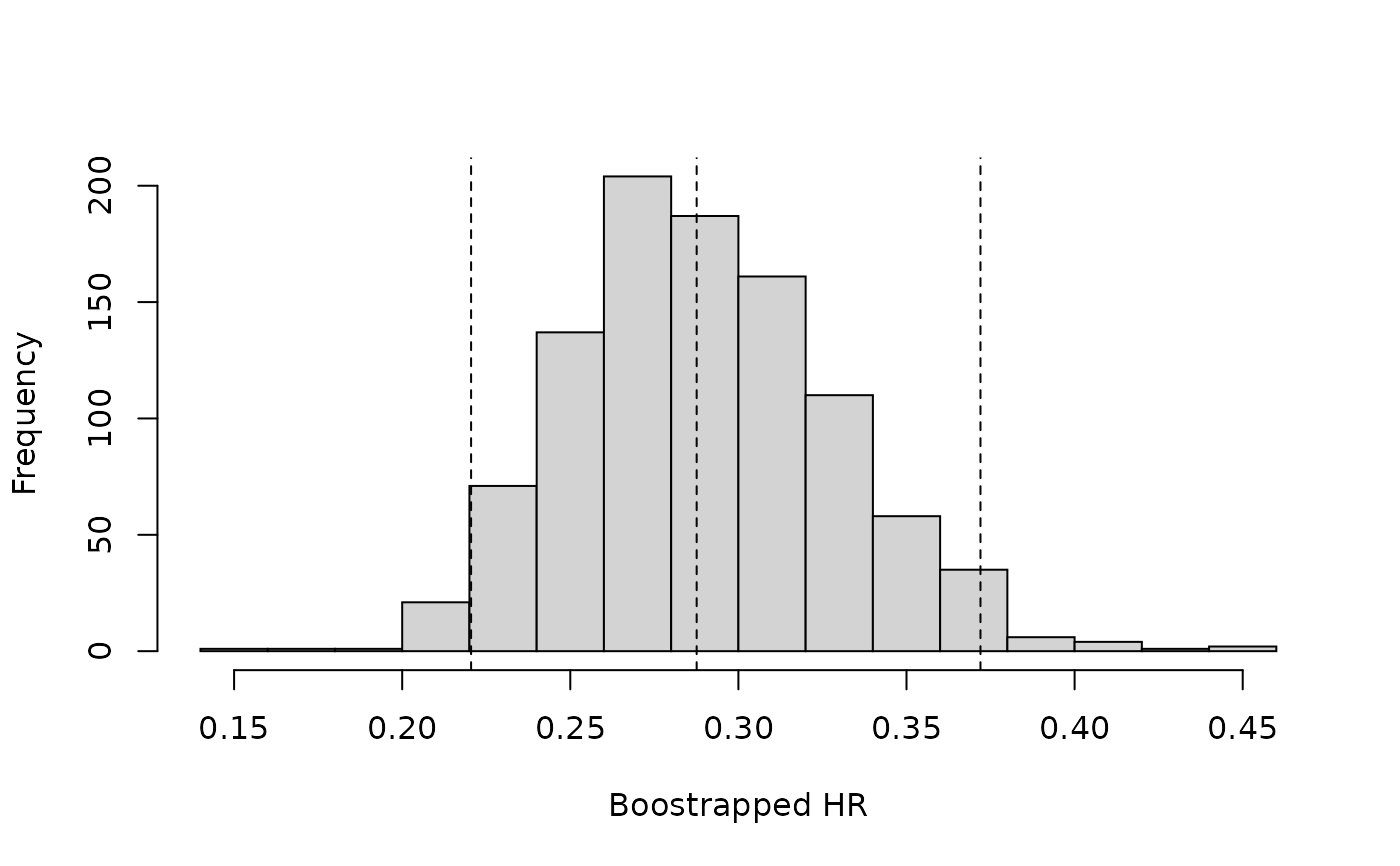
## Bootstrapping diagnostics
# Summarize bootstrap estimates in a histogram
# Vertical lines indicate the median and upper and lower CIs
hist(HR_bootstraps$t, main = "", xlab = "Boostrapped HR")
abline(v= quantile(HR_bootstraps$t, probs = c(0.025, 0.5, 0.975)), lty=2)
 # Median of the bootstrap samples
HR_median <- median(HR_bootstraps$t)
# Bootstrap CI - Percentile CI
boot_ci_HR <- boot.ci(boot.out = HR_bootstraps, index=1, type="perc")
# Bootstrap CI - BCa CI
boot_ci_HR_BCA <- boot.ci(boot.out = HR_bootstraps, index=1, type="bca")
## Summary
# Produce a summary of HRs and CIs
HR_summ <- rbind(HR_CI_cox, HR_CI_cox_wtd) %>% # Unweighted and weighted HRs and CIs from Cox models
mutate(Method = c("HR (95% CI) from unadjusted Cox model",
"HR (95% CI) from weighted Cox model")) %>%
# Median bootstrapped HR and 95% percentile CI
rbind(data.frame("HR" = HR_median,
"HR_low_CI" = boot_ci_HR$percent[4],
"HR_upp_CI" = boot_ci_HR$percent[5],
"Method"="Bootstrap median HR (95% percentile CI)")) %>%
# Median bootstrapped HR and 95% bias-corrected and accelerated bootstrap CI
rbind(data.frame("HR" = HR_median,
"HR_low_CI" = boot_ci_HR_BCA$bca[4],
"HR_upp_CI" = boot_ci_HR_BCA$bca[5],
"Method"="Bootstrap median HR (95% BCa CI)")) %>%
#apply rounding for numeric columns
mutate_if(.predicate = is.numeric, sprintf, fmt = "%.3f") %>%
#format for output
transmute(Method, HR_95_CI = paste0(HR, " (", HR_low_CI, " to ", HR_upp_CI, ")"))
# Summarize the results in a table suitable for word/ powerpoint
HR_table <- HR_summ %>%
regulartable() %>% #make it a flextable object
set_header_labels(Method = "Method", HR_95_CI = "Hazard ratio (95% CI)") %>%
font(font = 'Arial', part = 'all') %>%
fontsize(size = 14, part = 'all') %>%
bold(part = 'header') %>%
align(align = 'center', part = 'all') %>%
align(j = 1, align = 'left', part = 'all') %>%
border_outer(border = fp_border()) %>%
border_inner_h(border = fp_border()) %>%
border_inner_v(border = fp_border()) %>%
autofit(add_w = 0.2, add_h = 2)
### Example for response data --------------------------------------------------
## Estimating the odds ratio (OR)
# Fit a logistic regression model without weights to estimate the unweighted OR
unweighted_OR <- glm(formula = response~ARM,
family = binomial(link="logit"),
data = combined_data)
# Log odds ratio
log_OR_CI_logit <- cbind(coef(unweighted_OR), confint.default(unweighted_OR, level = 0.95))[2,]
# Exponentiate to get Odds ratio
OR_CI_logit <- exp(log_OR_CI_logit)
#tidy up naming
names(OR_CI_logit) <- c("OR", "OR_low_CI", "OR_upp_CI")
# Fit a logistic regression model with weights to estimate the weighted OR
weighted_OR <- suppressWarnings(glm(formula = response~ARM,
family = binomial(link="logit"),
data = combined_data,
weight = wt))
# Weighted log odds ratio
log_OR_CI_logit_wtd <- cbind(coef(weighted_OR), confint.default(weighted_OR, level = 0.95))[2,]
# Exponentiate to get weighted odds ratio
OR_CI_logit_wtd <- exp(log_OR_CI_logit_wtd)
#tidy up naming
names(OR_CI_logit_wtd) <- c("OR", "OR_low_CI", "OR_upp_CI")
## Bootstrap the confidence interval of the weighted OR
OR_bootstraps <- boot(data = est_weights$analysis_data, # intervention data
statistic = bootstrap_OR, # bootstrap the OR
R = 1000, # number of bootstrap samples
comparator_data = comparator_input, # comparator pseudo data
matching = est_weights$matching_vars, # matching variables
model = 'response ~ ARM' # model to fit
)
## Bootstrapping diagnostics
# Summarize bootstrap estimates in a histogram
# Vertical lines indicate the median and upper and lower CIs
hist(OR_bootstraps$t, main = "", xlab = "Boostrapped OR")
abline(v= quantile(OR_bootstraps$t, probs = c(0.025,0.5,0.975)), lty=2)
# Median of the bootstrap samples
HR_median <- median(HR_bootstraps$t)
# Bootstrap CI - Percentile CI
boot_ci_HR <- boot.ci(boot.out = HR_bootstraps, index=1, type="perc")
# Bootstrap CI - BCa CI
boot_ci_HR_BCA <- boot.ci(boot.out = HR_bootstraps, index=1, type="bca")
## Summary
# Produce a summary of HRs and CIs
HR_summ <- rbind(HR_CI_cox, HR_CI_cox_wtd) %>% # Unweighted and weighted HRs and CIs from Cox models
mutate(Method = c("HR (95% CI) from unadjusted Cox model",
"HR (95% CI) from weighted Cox model")) %>%
# Median bootstrapped HR and 95% percentile CI
rbind(data.frame("HR" = HR_median,
"HR_low_CI" = boot_ci_HR$percent[4],
"HR_upp_CI" = boot_ci_HR$percent[5],
"Method"="Bootstrap median HR (95% percentile CI)")) %>%
# Median bootstrapped HR and 95% bias-corrected and accelerated bootstrap CI
rbind(data.frame("HR" = HR_median,
"HR_low_CI" = boot_ci_HR_BCA$bca[4],
"HR_upp_CI" = boot_ci_HR_BCA$bca[5],
"Method"="Bootstrap median HR (95% BCa CI)")) %>%
#apply rounding for numeric columns
mutate_if(.predicate = is.numeric, sprintf, fmt = "%.3f") %>%
#format for output
transmute(Method, HR_95_CI = paste0(HR, " (", HR_low_CI, " to ", HR_upp_CI, ")"))
# Summarize the results in a table suitable for word/ powerpoint
HR_table <- HR_summ %>%
regulartable() %>% #make it a flextable object
set_header_labels(Method = "Method", HR_95_CI = "Hazard ratio (95% CI)") %>%
font(font = 'Arial', part = 'all') %>%
fontsize(size = 14, part = 'all') %>%
bold(part = 'header') %>%
align(align = 'center', part = 'all') %>%
align(j = 1, align = 'left', part = 'all') %>%
border_outer(border = fp_border()) %>%
border_inner_h(border = fp_border()) %>%
border_inner_v(border = fp_border()) %>%
autofit(add_w = 0.2, add_h = 2)
### Example for response data --------------------------------------------------
## Estimating the odds ratio (OR)
# Fit a logistic regression model without weights to estimate the unweighted OR
unweighted_OR <- glm(formula = response~ARM,
family = binomial(link="logit"),
data = combined_data)
# Log odds ratio
log_OR_CI_logit <- cbind(coef(unweighted_OR), confint.default(unweighted_OR, level = 0.95))[2,]
# Exponentiate to get Odds ratio
OR_CI_logit <- exp(log_OR_CI_logit)
#tidy up naming
names(OR_CI_logit) <- c("OR", "OR_low_CI", "OR_upp_CI")
# Fit a logistic regression model with weights to estimate the weighted OR
weighted_OR <- suppressWarnings(glm(formula = response~ARM,
family = binomial(link="logit"),
data = combined_data,
weight = wt))
# Weighted log odds ratio
log_OR_CI_logit_wtd <- cbind(coef(weighted_OR), confint.default(weighted_OR, level = 0.95))[2,]
# Exponentiate to get weighted odds ratio
OR_CI_logit_wtd <- exp(log_OR_CI_logit_wtd)
#tidy up naming
names(OR_CI_logit_wtd) <- c("OR", "OR_low_CI", "OR_upp_CI")
## Bootstrap the confidence interval of the weighted OR
OR_bootstraps <- boot(data = est_weights$analysis_data, # intervention data
statistic = bootstrap_OR, # bootstrap the OR
R = 1000, # number of bootstrap samples
comparator_data = comparator_input, # comparator pseudo data
matching = est_weights$matching_vars, # matching variables
model = 'response ~ ARM' # model to fit
)
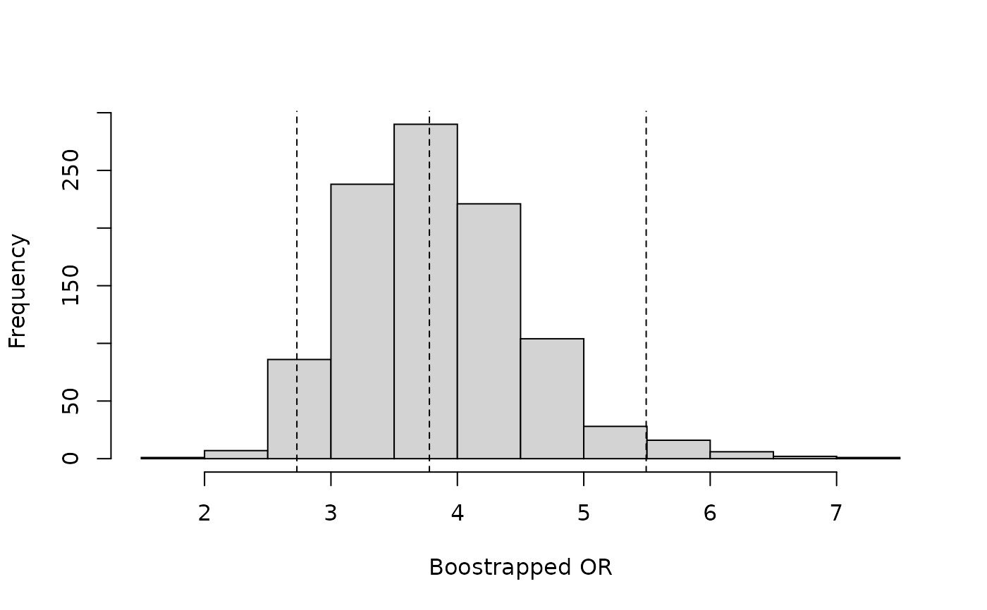
## Bootstrapping diagnostics
# Summarize bootstrap estimates in a histogram
# Vertical lines indicate the median and upper and lower CIs
hist(OR_bootstraps$t, main = "", xlab = "Boostrapped OR")
abline(v= quantile(OR_bootstraps$t, probs = c(0.025,0.5,0.975)), lty=2)
 # Median of the bootstrap samples
OR_median <- median(OR_bootstraps$t)
# Bootstrap CI - Percentile CI
boot_ci_OR <- boot.ci(boot.out = OR_bootstraps, index=1, type="perc")
# Bootstrap CI - BCa CI
boot_ci_OR_BCA <- boot.ci(boot.out = OR_bootstraps, index=1, type="bca")
## Summary
# Produce a summary of ORs and CIs
OR_summ <- rbind(OR_CI_logit, OR_CI_logit_wtd) %>% # Unweighted and weighted ORs and CIs
as.data.frame() %>%
mutate(Method = c("OR (95% CI) from unadjusted logistic regression model",
"OR (95% CI) from weighted logistic regression model")) %>%
# Median bootstrapped HR and 95% percentile CI
rbind(data.frame("OR" = OR_median,
"OR_low_CI" = boot_ci_OR$percent[4],
"OR_upp_CI" = boot_ci_OR$percent[5],
"Method"="Bootstrap median HR (95% percentile CI)")) %>%
# Median bootstrapped HR and 95% bias-corrected and accelerated bootstrap CI
rbind(data.frame("OR" = OR_median,
"OR_low_CI" = boot_ci_OR_BCA$bca[4],
"OR_upp_CI" = boot_ci_OR_BCA$bca[5],
"Method"="Bootstrap median HR (95% BCa CI)")) %>%
#apply rounding for numeric columns
mutate_if(.predicate = is.numeric, sprintf, fmt = "%.3f") %>%
#format for output
transmute(Method, OR_95_CI = paste0(OR, " (", OR_low_CI, " to ", OR_upp_CI, ")"))
# turns the results to a table suitable for word/ powerpoint
OR_table <- OR_summ %>%
regulartable() %>% #make it a flextable object
set_header_labels(Method = "Method", OR_95_CI = "Odds ratio (95% CI)") %>%
font(font = 'Arial', part = 'all') %>%
fontsize(size = 14, part = 'all') %>%
bold(part = 'header') %>%
align(align = 'center', part = 'all') %>%
align(j = 1, align = 'left', part = 'all') %>%
border_outer(border = fp_border()) %>%
border_inner_h(border = fp_border()) %>%
border_inner_v(border = fp_border()) %>%
autofit(add_w = 0.2)
# Median of the bootstrap samples
OR_median <- median(OR_bootstraps$t)
# Bootstrap CI - Percentile CI
boot_ci_OR <- boot.ci(boot.out = OR_bootstraps, index=1, type="perc")
# Bootstrap CI - BCa CI
boot_ci_OR_BCA <- boot.ci(boot.out = OR_bootstraps, index=1, type="bca")
## Summary
# Produce a summary of ORs and CIs
OR_summ <- rbind(OR_CI_logit, OR_CI_logit_wtd) %>% # Unweighted and weighted ORs and CIs
as.data.frame() %>%
mutate(Method = c("OR (95% CI) from unadjusted logistic regression model",
"OR (95% CI) from weighted logistic regression model")) %>%
# Median bootstrapped HR and 95% percentile CI
rbind(data.frame("OR" = OR_median,
"OR_low_CI" = boot_ci_OR$percent[4],
"OR_upp_CI" = boot_ci_OR$percent[5],
"Method"="Bootstrap median HR (95% percentile CI)")) %>%
# Median bootstrapped HR and 95% bias-corrected and accelerated bootstrap CI
rbind(data.frame("OR" = OR_median,
"OR_low_CI" = boot_ci_OR_BCA$bca[4],
"OR_upp_CI" = boot_ci_OR_BCA$bca[5],
"Method"="Bootstrap median HR (95% BCa CI)")) %>%
#apply rounding for numeric columns
mutate_if(.predicate = is.numeric, sprintf, fmt = "%.3f") %>%
#format for output
transmute(Method, OR_95_CI = paste0(OR, " (", OR_low_CI, " to ", OR_upp_CI, ")"))
# turns the results to a table suitable for word/ powerpoint
OR_table <- OR_summ %>%
regulartable() %>% #make it a flextable object
set_header_labels(Method = "Method", OR_95_CI = "Odds ratio (95% CI)") %>%
font(font = 'Arial', part = 'all') %>%
fontsize(size = 14, part = 'all') %>%
bold(part = 'header') %>%
align(align = 'center', part = 'all') %>%
align(j = 1, align = 'left', part = 'all') %>%
border_outer(border = fp_border()) %>%
border_inner_h(border = fp_border()) %>%
border_inner_v(border = fp_border()) %>%
autofit(add_w = 0.2)