Matching-Adjusted Indirect Comparison: Example using the <tt>MAIC</tt> package • MAIC

Introduction

This document describes the steps required to perform a matching-adjusted indirect comparison (MAIC) analysis using the MAIC package in R for a disconnected treatment network where the endpoint of interest is either time-to-event (e.g. overall survival) or binary (e.g. objective tumor response).

The methods described in this document are based on those originally described by Signorovitch et al. 2012 and described in the National Institute for Health and Care Excellence (NICE) Decision Support Unit (DSU) Technical Support Document (TSD) 18.[1,2]

MAIC methods are often required when:

There is no common comparator treatment to link a clinical trial of a new intervention to clinical trials of other treatments in a given disease area. For example if the only study of a new intervention is a single arm trial with no control group. This is commonly referred to as an unanchored MAIC.
A common comparator is available to link a clinical trial of a new intervention to a clinical trial of one other treatment in a given disease area but there are substantial differences in patient demographic or disease characteristics that are believed to be either prognostic or treatment effect modifiers. This is commonly referred to as an anchored MAIC.

The premise of MAIC methods is to adjust for between-trial differences in patient demographic or disease characteristics at baseline. When a common treatment comparator or ‘linked network’ are unavailable, a MAIC assumes that differences between absolute outcomes that would be observed in each trial are entirely explained by imbalances in prognostic variables and treatment effect modifiers. Prognostic variables are those that are predictive of disease outcomes, independent of the treatment received. For example, older patients may have increased risk of death compared to younger patients. Treatment effect modifiers are those variables that influence the relative effect of one treatment compared to another. For example patients with a better performance status may experience a larger treatment benefit than those with a worse performance status. Under this assumption, every prognostic variable and every treatment effect modifier that is imbalanced between the two studies must be available. This assumption is generally considered very difficult to meet.[2] There are several ways of identifying prognostic variables/treatment effect modifiers to be used in the MAIC analyses, some of which include:

Clinical expertise (when available to a project)
Published papers/previous submissions (what has been identified in the disease area previously)
Univariable/multivariable regression analyses to identify which covariates have a significant effect on the outcome
Subgroup analyses of clinical trials may identify interactions between patient characteristics and the relative treatment effect

Example Scenario

For the purposes of this example, we present an unanchored MAIC of two treatments in lung cancer with the treatments being compared labelled ‘intervention’ and ‘comparator.’ The two endpoints being compared are overall survival (a time to event outcome) and objective response (a binary outcome). The data used in this example have been simulated to resemble that of clinical trial data. The data available are:

Individual patient data from a single arm study of ‘intervention’
Aggregate summary data for ‘comparator.’ This could be from a single arm study of the comparator or from one arm of a randomized controlled trial.
Psuedo patient data from the comparator study. This is not required for the matching process but is needed to derive the relative treatment effects between the intervention and comparator.

In this example scenario, age, sex, the Eastern Cooperative Oncology Group performance status (ECOG PS) and smoking status have been identified as imbalanced prognostic variables/treatment effect modifiers.

Set up packages and data

Install packages

The following packages are required to run this example:

library(dplyr)
library(boot)
library(survival)
library(MAIC)
library(ggplot2)
library(survminer)
library(flextable)
library(officer)
# set seed to give reproducible example
set.seed(1894)

Read in the data

To perform unanchored MAICs, the following data is required:

Individual patient data (IPD) from the intervention trial
Baseline data from the comparator trial
Pseudo data for the comparator trial (see Comparator pseudo data)

Simulated data for the above is provided with the MAIC package.

Intervention trial IPD

This example reads in and combines data from three standard simulated data sets (adsl, adrs and adtte) which are saved as ‘.csv’ files. The data may need some manipulation to standardize the variable names to ensure they are the same in all datasets.

The variables needed for the time to event analyses are:

Time - a numeric variable
Event - a binary variable (event=1, censor=0)
Treatment - a character variable with the name of the intervention treatment

The variables needed for the binary event analyses are:

Response - a binary variable (event=1, no event=0)
Treatment - a character variable with the name of the intervention treatment

For the matching variables:

All binary variables to be used in the matching should be coded 1 and 0 (see example for sex below).
The variable names need to be listed in a character vector called match_cov.

#### Intervention data

# Read in ADaM data and rename variables of interest

adsl <- read.csv(system.file("extdata", "adsl.csv", package = "MAIC", mustWork = TRUE))
adrs <- read.csv(system.file("extdata", "adrs.csv", package = "MAIC", mustWork = TRUE))
adtte <- read.csv(system.file("extdata", "adtte.csv", package = "MAIC", mustWork = TRUE))

adsl <- adsl %>% # Data containing the matching variables
   mutate(SEX=ifelse(SEX=="Male", 1, 0)) # Coded 1 for males and 0 for females

adrs <- adrs %>% # Response data
   filter(PARAM=="Response") %>%
   transmute(USUBJID, ARM, response=AVAL)

adtte <- adtte %>% # Time to event data (overall survival)
   filter(PARAMCD=="OS") %>%
   mutate(Event=1-CNSR) %>% #Set up coding as Event = 1, Censor = 0
   transmute(USUBJID, ARM, Time=AVAL, Event)

# Combine all intervention data
intervention_input <- adsl %>%
  full_join(adrs, by=c("USUBJID", "ARM")) %>%
  full_join(adtte, by=c("USUBJID", "ARM"))
head(intervention_input)
#>   USUBJID ARM AGE SEX SMOKE ECOG0 response     Time Event
#> 1       1   A  45   1     0     0        0 281.5195     0
#> 2       2   A  71   1     0     0        1 500.0000     0
#> 3       3   A  58   1     1     1        1 304.6406     0
#> 4       4   A  48   0     0     1        1 102.4731     0
#> 5       5   A  69   1     0     1        0 101.6632     0
#> 6       6   A  48   0     0     1        0 237.0593     1

# List out matching covariates
match_cov <- c("AGE",
               "SEX",
               "SMOKE",
               "ECOG0")

Baseline data from the comparator trial

The aggregate baseline characteristics (number of patients, mean and SD for continuous variables and proportion for binary variables) from the comparator trial are needed as a data frame. Naming of the covariates in this data frame (named below as target_pop_standard) should be consistent with the intervention data (intervention_input).

# Baseline aggregate data for the comparator population
target_pop <- read.csv(system.file("extdata", "aggregate_data.csv",
                                   package = "MAIC", mustWork = TRUE))

# Renames target population cols to be consistent with match_cov
match_cov
#> [1] "AGE"   "SEX"   "SMOKE" "ECOG0"
names(target_pop)
#>  [1] "N"          "age.mean"   "age.sd"     "N.male"     "prop.male" 
#>  [6] "N.ecog0"    "prop.ecog0" "N.smoke"    "prop.smoke" "ARM"
target_pop_standard <- target_pop %>%
  #EDIT
   rename(N=N,
          Treatment=ARM,
          AGE=age.mean,
          SEX=prop.male,
          SMOKE=prop.smoke,
          ECOG0=prop.ecog0
  ) %>%
  transmute(N, Treatment, AGE, SEX, SMOKE, ECOG0)

target_pop_standard
#>     N  Treatment      AGE  SEX     SMOKE ECOG0
#> 1 300 Comparator 50.06333 0.49 0.1933333  0.35

Estimate weights

Statistical theory

As described by Signorovitch et al. (supplemental appendix), we must find a \(\beta\), such that re-weighting baseline characteristics for the intervention, \(x_{i,ild}\) exactly matches the mean baseline characteristics for the comparator data source for which only aggregate data is available.[1]

The weights are given by: \[\hat{\omega}_i=\exp{(x_{i,ild}.\beta)}\qquad (1)\] That is, we must find a solution to: \[ \bar{x}_{agg}\sum_{i=1}^n \exp{(x_{i,ild}.\beta)} = \sum_{i=1}^n x_{i,ild}.\exp{(x_{i,ild}.\beta)}\qquad (2) \] This estimator is equivalent to solving the equation \[ 0 = \sum_{i=1}^n (x_{i,ild} - \bar{x}_{agg} ).\exp{(x_{i,ild}.\beta)}\qquad (3)\] without loss of generality, it can be assumed that \(\bar{x}_{agg} = 0\) (e.g we could transform baseline characteristics in both trials by subtracting \(\bar{x}_{agg}\)) leaving the estimator \[0 = \sum_{i=1}^n (x_{i,ild})\exp{(x_{i,ild}.\beta)}\qquad (4)\] The right hand side of this estimator is the first derivative of \[ Q(\beta) = \sum_{i=1}^n \exp{(x_{i,ild}.\beta)}\qquad (5) \] As described by Signorovitch et al (supplemental appendix), \(Q(\beta)\) is convex and therefore any finite solution to (2) is unique and corresponds to the global minimum of \(Q(\beta)\).

In order to facilitate estimation of patient weights, \(\hat{\omega}_i\), it is necessary to center the baseline characteristics of the intervention data using the mean baseline characteristics from the comparator data.

As described by Phillippo, balancing on both mean and standard deviation for continuous variables (where possible) may be considered in some cases. This is included in the example below.[2]

The code below also specifies an object (cent_match_cov) that contains the names of the centered matching variables - this will be needed for the analyses below.

#### center baseline characteristics
# (subtract the aggregate comparator data from the corresponding column of intervention PLD)
names(intervention_input)
#> [1] "USUBJID"  "ARM"      "AGE"      "SEX"      "SMOKE"    "ECOG0"    "response"
#> [8] "Time"     "Event"

intervention_data <- intervention_input %>%
         mutate(Age_centered = AGE - target_pop$age.mean,
                # matching on both mean and standard deviation for continuous variable (optional)
                Age_squared_centered = (AGE^2) - (target_pop$age.mean^2 + target_pop$age.sd^2),
                Sex_centered = SEX - target_pop$prop.male,
                Smoke_centered = SMOKE - target_pop$prop.smoke,
                ECOG0_centered = ECOG0 - target_pop$prop.ecog0)

head(intervention_data)
#>   USUBJID ARM AGE SEX SMOKE ECOG0 response     Time Event Age_centered
#> 1       1   A  45   1     0     0        0 281.5195     0    -5.063333
#> 2       2   A  71   1     0     0        1 500.0000     0    20.936667
#> 3       3   A  58   1     1     1        1 304.6406     0     7.936667
#> 4       4   A  48   0     0     1        1 102.4731     0    -2.063333
#> 5       5   A  69   1     0     1        0 101.6632     0    18.936667
#> 6       6   A  48   0     0     1        0 237.0593     1    -2.063333
#>   Age_squared_centered Sex_centered Smoke_centered ECOG0_centered
#> 1            -491.8049         0.51     -0.1933333          -0.35
#> 2            2524.1951         0.51     -0.1933333          -0.35
#> 3             847.1951         0.51      0.8066667           0.65
#> 4            -212.8049        -0.49     -0.1933333           0.65
#> 5            2244.1951         0.51     -0.1933333           0.65
#> 6            -212.8049        -0.49     -0.1933333           0.65

# Set matching covariates
cent_match_cov <- c("Age_centered",
                    "Age_squared_centered",
                    "Sex_centered",
                    "Smoke_centered",
                    "ECOG0_centered")

Optimization procedure

Following the centering of the baseline characteristics of the intervention study, patient weights can be estimated using the estimate_weights function in the MAIC package. This performs an optimization procedure to minimize \(Q(\beta) = \sum_{i=1}^n \exp{(x_{i,ild}.\beta)}\) and outputs a list containing:

A character vector containing the names of the matching variables
An analysis data frame of the intervention data with weights

est_weights <- estimate_weights(intervention_data = intervention_data,
                                matching_vars = cent_match_cov)

head(est_weights$analysis_data)
#>   USUBJID          ARM AGE SEX SMOKE ECOG0 response     Time Event Age_centered
#> 1       1 Intervention  45   1     0     0        0 281.5195     0    -5.063333
#> 2       2 Intervention  71   1     0     0        1 500.0000     0    20.936667
#> 3       3 Intervention  58   1     1     1        1 304.6406     0     7.936667
#> 4       4 Intervention  48   0     0     1        1 102.4731     0    -2.063333
#> 5       5 Intervention  69   1     0     1        0 101.6632     0    18.936667
#> 6       6 Intervention  48   0     0     1        0 237.0593     1    -2.063333
#>   Age_squared_centered Sex_centered Smoke_centered ECOG0_centered           wt
#> 1            -491.8049         0.51     -0.1933333          -0.35 1.301506e+00
#> 2            2524.1951         0.51     -0.1933333          -0.35 7.024764e-08
#> 3             847.1951         0.51      0.8066667           0.65 6.384284e-02
#> 4            -212.8049        -0.49     -0.1933333           0.65 1.204094e+00
#> 5            2244.1951         0.51     -0.1933333           0.65 1.371621e-06
#> 6            -212.8049        -0.49     -0.1933333           0.65 1.204094e+00
#>          wt_rs
#> 1 3.457953e+00
#> 2 1.866400e-07
#> 3 1.696231e-01
#> 4 3.199141e+00
#> 5 3.644239e-06
#> 6 3.199141e+00

est_weights$matching_vars
#> [1] "Age_centered"         "Age_squared_centered" "Sex_centered"        
#> [4] "Smoke_centered"       "ECOG0_centered"

Weight diagnostics

Following the calculation of weights, it is necessary to determine whether the optimization procedure has worked correctly and whether the weights derived are sensible.

Are the weights sensible?

Effective sample size

For a weighted estimate, the effective sample size (ESS) is the number of independent non-weighted individuals that would be required to give an estimate with the same precision as the weighted sample estimate. The approximate effective sample size is calculated as: \[ ESS = \frac{({ \sum_{i=1}^n \hat{\omega}_i })^2}{ \sum_{i=1}^n \hat{\omega^2}_i } \] A small ESS, relative to the original sample size, is an indication that the weights are highly variable and that the estimate may be unstable. This often occurs if there is very limited overlap in the distribution of the matching variables between the populations being compared. If there is insufficient overlap between populations it may not be possible to obtain reliable estimates of the weights

The MAIC package includes a function to estimate the ESS:

ESS <- estimate_ess(est_weights$analysis_data)
ESS
#> [1] 157.0715

In this example, the ESS is 31% of the total number of patients in the intervention arm (500 patients in total). As this is a considerable reduction from the total number of patients, estimates using this weighted data may be unreliable. The reliability of the estimate could be explored by considering matching on a subset of the matching variables, for example, those considered most important. However, unless all prognostic factors and effect modifiers are included in the adjustment, the estimates will remain biased.[2,3]

Rescaled weights

It is easier to examine the distribution of the weights by scaling them, so that the rescaled weights are relative to the original unit weights of each individual. In other words, a rescaled weight \(>\) 1 means that an individual carries more weight in the re-weighted population than the original data and a rescaled weight \(<\) 1 means that an individual carries less weight in the re-weighted population than the original data. The rescaled weights are calculated as:

\[\tilde{\omega}_i = \frac{ \hat{\omega}_i}{ \sum_{i=1}^n \hat{\omega}_i }.N \]

A histogram of the rescaled weights (along with a histogram of the weights) can be produced using the hist_wts function in the MAIC package. bin_width needs to be adapted depending on the sample size in the data set by using the bin statement.

# Plot histograms of unscaled and rescaled weights
# bin_width needs to be adapted depending on the sample size in the data set
histogram <- hist_wts(est_weights$analysis_data, bin = 50)
histogram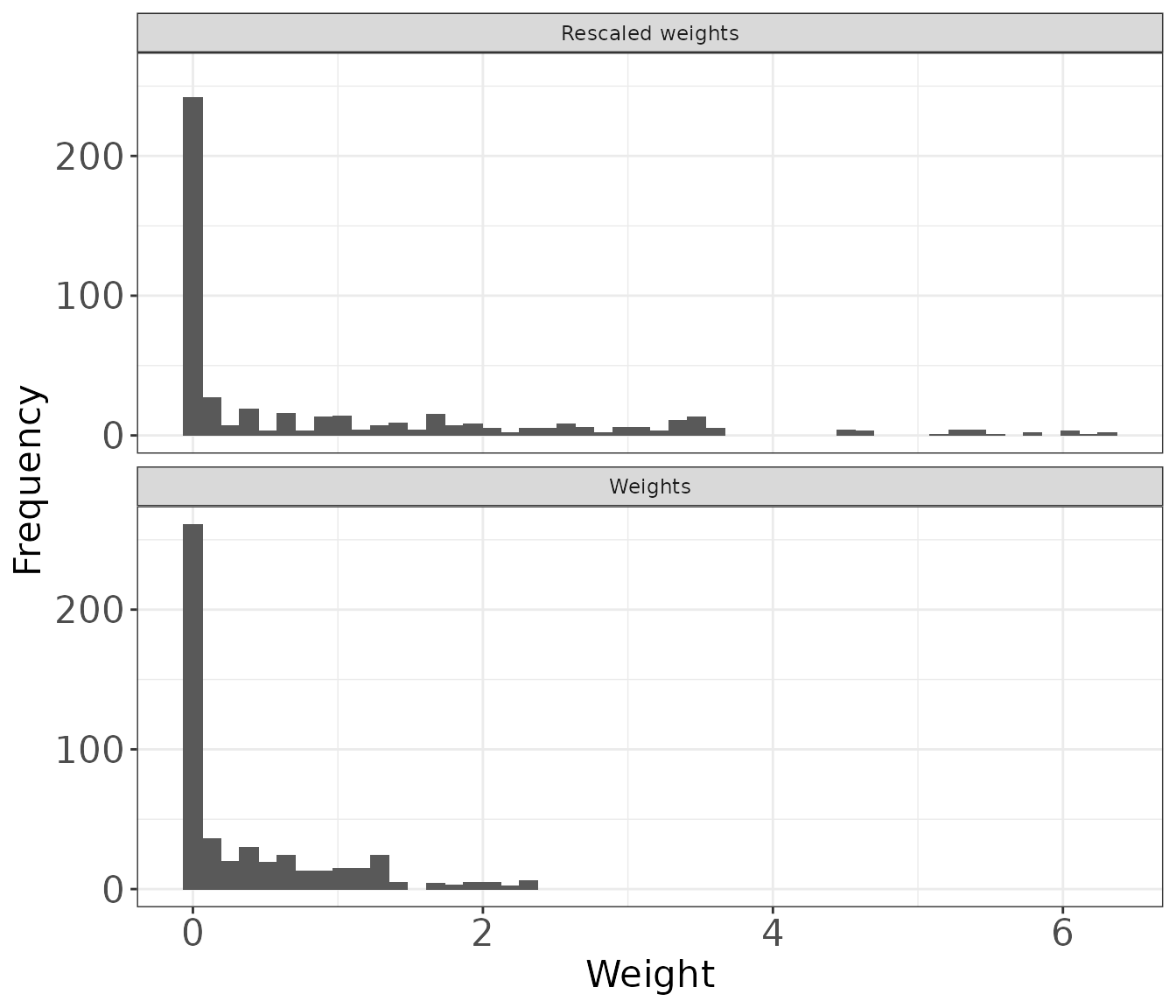

The distribution of rescaled weights can be further explored by producing a summary of the mean, standard deviation, median, minimum and maximum rescaled weight. The MAIC package includes the summarize_wts function to produce this summary for the rescaled weights and the weights.

weight_summ <- summarize_wts(est_weights$analysis_data)
weight_summ
#>               type      mean       sd     median          min      max
#> 1          Weights 0.3763805 0.556692 0.03467630 1.855194e-11 2.373310
#> 2 Rescaled weights 1.0000000 1.479067 0.09213098 4.929037e-11 6.305614

To understand which individuals are carrying more or less weight in the re-weighted population than the original data the profile_wts function in the MAIC package creates a data set with a unique set of weights and the corresponding patient profile based on the matching variables. When matching on a continuous variable there will be multiple unique weights and the output from this function is less useful. When there is a small set of unique weights profile_wts is useful to describe those patients who have more or less influence on the weighted analyses.

wts_profile <- profile_wts(est_weights$analysis_data, vars = match_cov)
head(wts_profile)
#>   AGE SEX SMOKE ECOG0           wt        wt_rs
#> 1  45   1     0     0 1.301506e+00 3.457953e+00
#> 2  71   1     0     0 7.024764e-08 1.866400e-07
#> 3  58   1     1     1 6.384284e-02 1.696231e-01
#> 4  48   0     0     1 1.204094e+00 3.199141e+00
#> 5  69   1     0     1 1.371621e-06 3.644239e-06
#> 6  47   1     1     0 1.010290e+00 2.684226e+00

Overall weight diagnostics summary function

To quickly produce the weight diagnostics, the MAIC package includes the function wt_diagnostics which brings together the three functions:

ESS
weight_summ
wts_profile

# Function to produce a set of diagnostics.
# Calls each of the diagnostic functions above except for plotting histograms
diagnostics <- wt_diagnostics(est_weights$analysis_data, vars = match_cov)

diagnostics$ESS
#> [1] 157.0715

diagnostics$Summary_of_weights
#>               type      mean       sd     median          min      max
#> 1          Weights 0.3763805 0.556692 0.03467630 1.855194e-11 2.373310
#> 2 Rescaled weights 1.0000000 1.479067 0.09213098 4.929037e-11 6.305614
head(diagnostics$Weight_profiles)
#>   AGE SEX SMOKE ECOG0           wt        wt_rs
#> 1  45   1     0     0 1.301506e+00 3.457953e+00
#> 2  71   1     0     0 7.024764e-08 1.866400e-07
#> 3  58   1     1     1 6.384284e-02 1.696231e-01
#> 4  48   0     0     1 1.204094e+00 3.199141e+00
#> 5  69   1     0     1 1.371621e-06 3.644239e-06
#> 6  47   1     1     0 1.010290e+00 2.684226e+00

Has the optimization worked?

The following code checks whether the re-weighted baseline characteristics for the intervention-treated patients match those aggregate characteristics from the comparator trial and outputs a summary that can be used for reporting.

# Create an object to hold the output
baseline_summary <- list('Intervention' = NA, 
                         'Intervention_weighted' = NA, 
                         'Comparator' = NA)

# Summarise matching variables for weighted intervention data
baseline_summary$Intervention_weighted <- est_weights$analysis_data %>%
   transmute(AGE, SEX, SMOKE, ECOG0, wt) %>%
   summarise_at(match_cov, list(~ weighted.mean(., wt)))

# Summarise matching variables for unweighted intervention data
baseline_summary$Intervention <- est_weights$analysis_data %>%
   transmute(AGE, SEX, SMOKE, ECOG0, wt) %>%
   summarise_at(match_cov, list(~ mean(.)))

# baseline data for the comparator study
baseline_summary$Comparator <- transmute(target_pop_standard, AGE, SEX, SMOKE, ECOG0)

# Combine the three summaries
# Takes a list of data frames and binds these together
trt <- names(baseline_summary)

baseline_summary <- bind_rows(baseline_summary) %>%
  transmute_all(sprintf, fmt = "%.2f") %>% #apply rounding for presentation
  transmute(ARM = as.character(trt), AGE, SEX, SMOKE, ECOG0)

# Insert N of intervention  as number of patients
baseline_summary$`N/ESS`[baseline_summary$ARM == "Intervention"] <- nrow(est_weights$analysis_data)

# Insert N for comparator from target_pop_standard
baseline_summary$`N/ESS`[baseline_summary$ARM == "Comparator"] <- target_pop_standard$N

# Insert the ESS as the sample size for the weighted data
# This is calculated above but can also be obtained using the estimate_ess function as shown below
baseline_summary$`N/ESS`[baseline_summary$ARM == "Intervention_weighted"] <- est_weights$analysis_data %>%
  estimate_ess(wt_col = 'wt')

baseline_summary <- baseline_summary %>%
  transmute(ARM, `N/ESS`=round(`N/ESS`,1), AGE, SEX, SMOKE, ECOG0)
baseline_summary
#>                     ARM N/ESS   AGE  SEX SMOKE ECOG0
#> 1          Intervention 500.0 59.85 0.38  0.32  0.41
#> 2 Intervention_weighted 157.1 50.06 0.49  0.19  0.35
#> 3            Comparator 300.0 50.06 0.49  0.19  0.35

Incorporation of the weights in statistical analysis

Comparator pseudo data

Individual patient data was not available for the comparator study, therefore, pseudo individual patient data is required for these analyses to derive the relative treatment effects. These patients are given a weight of 1 for use in the weighted analysis.

Pseudo overall survival data was obtained for the comparator treatment by digitizing a reported overall survival Kaplan-Meier graph using the methodology of Guyot et al.[4] It is common for binary endpoints to be reported as a percentage of patients with the event and therefore the example code below simulates pseudo-data for objective response based on the total number of patients and the proportion of responders.

The comparator data will include pseudo individual patient data from two different endpoints and it should be highlighted that there is no 1:1 relationship between endpoints for a given patient since these are reconstructed data and not actual observed data.

Naming of variables in the comparator data should be consistent with those used in the intervention IPD.

#### Comparator pseudo data

# Read in digitised pseudo survival data, col names must match intervention_input
comparator_surv <- read.csv(system.file("extdata", "psuedo_IPD.csv",
                                        package = "MAIC", mustWork = TRUE)) %>%
  rename(Time=Time, Event=Event)


# Simulate response data based on the known proportion of responders
comparator_n <- nrow(comparator_surv) # total number of patients in the comparator data
comparator_prop_events <- 0.4 # proportion of responders
# Calculate number with event
# Use round() to ensure we end up with a whole number of people
# number without an event = Total N - number with event to ensure we keep the same number of patients
n_with_event <- round(comparator_n*comparator_prop_events, digits = 0)
comparator_binary <- data.frame("response"= c(rep(1, n_with_event), rep(0, comparator_n - n_with_event)))

# Join survival and response comparator data
# (note the rows do not represent observations from a particular patient)
comparator_input <- cbind(comparator_surv, comparator_binary) %>%
                    mutate(wt=1, wt_rs=1, ARM="Comparator") # All patients have weight = 1
head(comparator_input)
#>         Time Event response wt wt_rs        ARM
#> 1 20.2311676     1        1  1     1 Comparator
#> 2 28.7679537     1        1  1     1 Comparator
#> 3 41.0662129     0        1  1     1 Comparator
#> 4  0.8492261     1        1  1     1 Comparator
#> 5  9.0521882     0        1  1     1 Comparator
#> 6  3.4450075     1        1  1     1 Comparator


# Join comparator data with the intervention data
# Set factor levels to ensure "Comparator" is the reference treatment
combined_data <-  bind_rows(est_weights$analysis_data, comparator_input)
combined_data$ARM <- relevel(as.factor(combined_data$ARM), ref="Comparator")

Estimating the relative effect

Using the weights (not the rescaled weights) derived above, relative effects can be estimated using:

coxph for time to event endpoints via the use of the weights statement to estimate a weighted HR from a Cox proportional hazards model
glm for binary endpoints via the use of the weight statement to estimate a weighted OR from logistic regression

It is important to report the weighted relative effect with the unweighted relative effect to understand how the weighting has affected the analysis.

Bootstrapping a confidence interval

The use of weights induces a within-subject correlation in outcomes, as observations can have weights that are unequal to one another [5,6]. As such, it is necessary to use a variance estimator to take into account the lack of independence of observations. The two common approaches to this are robust variance estimation and bootstrapping. A simulation study was conducted by Austin et al to examine the different methods in the context of an inverse probability of treatment weighting (IPTW) survival analysis. The author concluded that the use of a bootstrap estimator resulted in approximately correct estimates of standard errors and confidence intervals with the correct coverage rate. The other estimators resulted in biased estimates of standard errors and confidence intervals with incorrect coverage rates. The use of a bootstrap type estimator is also intuitively appealing, a robust estimator assumes that the weights are known and not subject to any sampling uncertainty. However, a bootstrap estimator allows for quantification of the uncertainty in the estimation of the weights.

Bootstrapping involves:

Sampling, with replacement, from the patients in the intervention arm (a bootstrap sample)
Estimating a set of weights for each of these bootstrapped data sets and
Estimating a hazard ratio (HR)/odds ratio (OR) using each set of estimated weights.

This procedure is repeated multiple times to obtain a distribution of HRs/ORs. For this example, bootstrap estimates of the HRs/ORs were calculated using the boot package. An argument for the boot function is statistic which is a function which when applied to data returns a vector containing the statistic(s) of interest. The bootstrap_HR and bootstrap_OR in the MAIC package can be used for this purpose.

Two different methods for estimating a 95% confidence interval (CI) from the bootstrap samples were explored:[7–9]

Percentile CIs
- This method takes the 2.5th and 97.5th percentiles and can be implemented using the type=“perc” statement in the boot.ci function
Bias-corrected and accelerated (BCa) CIs
- This method attempts to correct for any bias and skewness in the distribution of bootstrap estimates and can be implemented using type=“bca” statement in the boot.ci function)
- The BCa method also takes percentiles but they are not necessarily the 2.5th and 97.5th percentiles (the choice of percentiles depends on an acceleration parameter [estimated through jackknife re-sampling] and a bias correction factor [proportion of bootstrap estimates less than the original estimator])

Example for survival data

Kaplan-Meier plot

To visualize the effect of the weighting compared to the unadjusted data, it is useful to plot a Kaplan-Meier. The figure below shows there is a clear treatment benefit of the intervention compared to the comparator. The treatment effect increases once the data is weighted. This treatment effect is quantified in the next section.

To note, the number of patients at the start of the Kaplan-Meier plot in the weighted population is equivalent to the sum of the weights. This will be different to the ESS.

# Unweighted intervention data
KM_int <- survfit(formula = Surv(Time, Event==1) ~ 1 ,
                  data = est_weights$analysis_data,
                  type="kaplan-meier")
# Weighted intervention data
KM_int_wtd <- survfit(formula = Surv(Time, Event==1) ~ 1 ,
                  data = est_weights$analysis_data,
                  weights = wt,
                  type="kaplan-meier")
# Comparator data
KM_comp <- survfit(formula = Surv(Time, Event==1) ~ 1 ,
                  data = comparator_input,
                  type="kaplan-meier")

# Combine the survfit objects ready for ggsurvplot
KM_list <- list(Intervention = KM_int,
                Intervention_weighted = KM_int_wtd,
                Comparator = KM_comp)

#Produce the Kaplan-Meier plot
KM_plot <- ggsurvplot(KM_list,
                      combine = TRUE,
                      risk.table=TRUE, # numbers at risk displayed on the plot
                      break.x.by=50,
                      xlab="Time (days)",
                      censor=FALSE,
                      legend.title = "Treatment",
                      title = "Kaplan-Meier plot of overall survival",
                      legend.labs=c("Intervention", "Intervention weighted", "Comparator"),
                      font.legend = list(size = 10)) +
                      guides(colour=guide_legend(nrow = 2))
KM_plot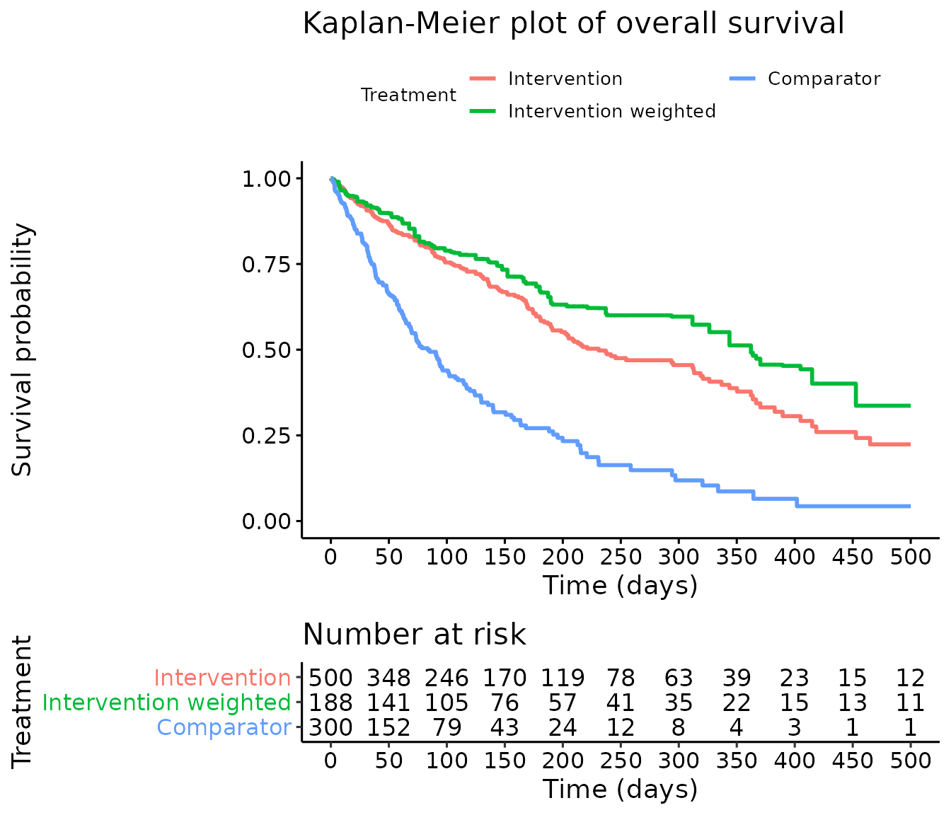

Estimating the hazard ratio (HR)

In this example, the weighted HR 0.29 (95% CI: 0.21, 0.40) shows a larger treatment effect (HR further from 1) than the unweighted HR 0.38 (95% CI: 0.30, 0.46). The median of the bootstrap HR samples is the same as the HR from the weighted Cox model to two decimal places (HR is 0.29). In this example, the percentile CI (0.22, 0.37) and BCa confidence interval (0.22, 0.37) are identical to two decimal places suggesting the bootstrap samples are relatively normally distributed (see diagnostics). Finally, it should be noted that results are relatively consistent across all methods, the intervention treatment significantly reduces the hazard of death compared with the comparator treatment.

## Calculate HRs

# Fit a Cox model without weights to estimate the unweighted HR
unweighted_cox <- coxph(Surv(Time, Event==1) ~ ARM, data = combined_data)

HR_CI_cox <- summary(unweighted_cox)$conf.int %>%
  as.data.frame() %>%
  transmute("HR" = `exp(coef)`, "HR_low_CI" = `lower .95`, "HR_upp_CI" = `upper .95`)

HR_CI_cox
#>                        HR HR_low_CI HR_upp_CI
#> ARMIntervention 0.3748981  0.303901 0.4624815

# Fit a Cox model with weights to estimate the weighted HR
weighted_cox <- coxph(Surv(Time, Event==1) ~ ARM, data = combined_data, weights = wt)

HR_CI_cox_wtd <- summary(weighted_cox)$conf.int %>%
  as.data.frame() %>%
  transmute("HR" = `exp(coef)`, "HR_low_CI" = `lower .95`, "HR_upp_CI" = `upper .95`)

HR_CI_cox_wtd
#>                        HR HR_low_CI HR_upp_CI
#> ARMIntervention 0.2864753 0.2072051 0.3960718

## Bootstrapping

# Bootstrap 1000 HRs
HR_bootstraps <- boot(data = est_weights$analysis_data, # intervention data
                      statistic = bootstrap_HR, # bootstrap the HR (defined in the MAIC package)
                      R=1000, # number of bootstrap samples
                      comparator_data = comparator_input, # comparator pseudo data
                      matching = est_weights$matching_vars, # matching variables
                      model = Surv(Time, Event==1) ~ ARM # model to fit
                      )

# Median of the bootstrap samples
HR_median <- median(HR_bootstraps$t)

# Bootstrap CI - Percentile CI
boot_ci_HR <- boot.ci(boot.out = HR_bootstraps, index=1, type="perc")

# Bootstrap CI - BCa CI
boot_ci_HR_BCA <- boot.ci(boot.out = HR_bootstraps, index=1, type="bca")

## Summary

# Produce a summary of HRs and CIs
HR_summ <-  rbind(HR_CI_cox, HR_CI_cox_wtd) %>% # Unweighted and weighted HRs and CIs from Cox models
  mutate(Method = c("HR (95% CI) from unadjusted Cox model",
                    "HR (95% CI) from weighted Cox model")) %>%

  # Median bootstrapped HR and 95% percentile CI
  rbind(data.frame("HR" = HR_median,
                   "HR_low_CI" = boot_ci_HR$percent[4],
                   "HR_upp_CI" = boot_ci_HR$percent[5],
                   "Method"="Bootstrap median HR (95% percentile CI)")) %>%

  # Median bootstrapped HR and 95% bias-corrected and accelerated bootstrap CI
  rbind(data.frame("HR" = HR_median,
                   "HR_low_CI" = boot_ci_HR_BCA$bca[4],
                   "HR_upp_CI" = boot_ci_HR_BCA$bca[5],
                   "Method"="Bootstrap median HR (95% BCa CI)")) %>%
  #apply rounding for numeric columns
  mutate_if(.predicate = is.numeric, sprintf, fmt = "%.3f") %>%
  #format for output
  transmute(Method, HR_95_CI = paste0(HR, " (", HR_low_CI, " to ", HR_upp_CI, ")"))

# turns the results to a table suitable for word/ powerpoint
HR_table <- HR_summ %>%
  regulartable() %>% #make it a flextable object
  set_header_labels(Method = "Method",  HR_95_CI = "Hazard ratio (95% CI)")  %>%
  font(font = 'Arial', part = 'all') %>%
  fontsize(size = 14, part = 'all') %>%
  bold(part = 'header') %>%
  align(align = 'center', part = 'all') %>%
  align(j = 1, align = 'left', part = 'all') %>%
  border_outer(border = fp_border()) %>%
  border_inner_h(border = fp_border()) %>%
  border_inner_v(border = fp_border()) %>%
  autofit(add_w = 0.2, add_h = 2)

HR_table

Method	Hazard ratio (95% CI)
HR (95% CI) from unadjusted Cox model	0.375 (0.304 to 0.462)
HR (95% CI) from weighted Cox model	0.286 (0.207 to 0.396)
Bootstrap median HR (95% percentile CI)	0.289 (0.218 to 0.369)
Bootstrap median HR (95% BCa CI)	0.289 (0.215 to 0.367)

Bootstrapping diagnostics

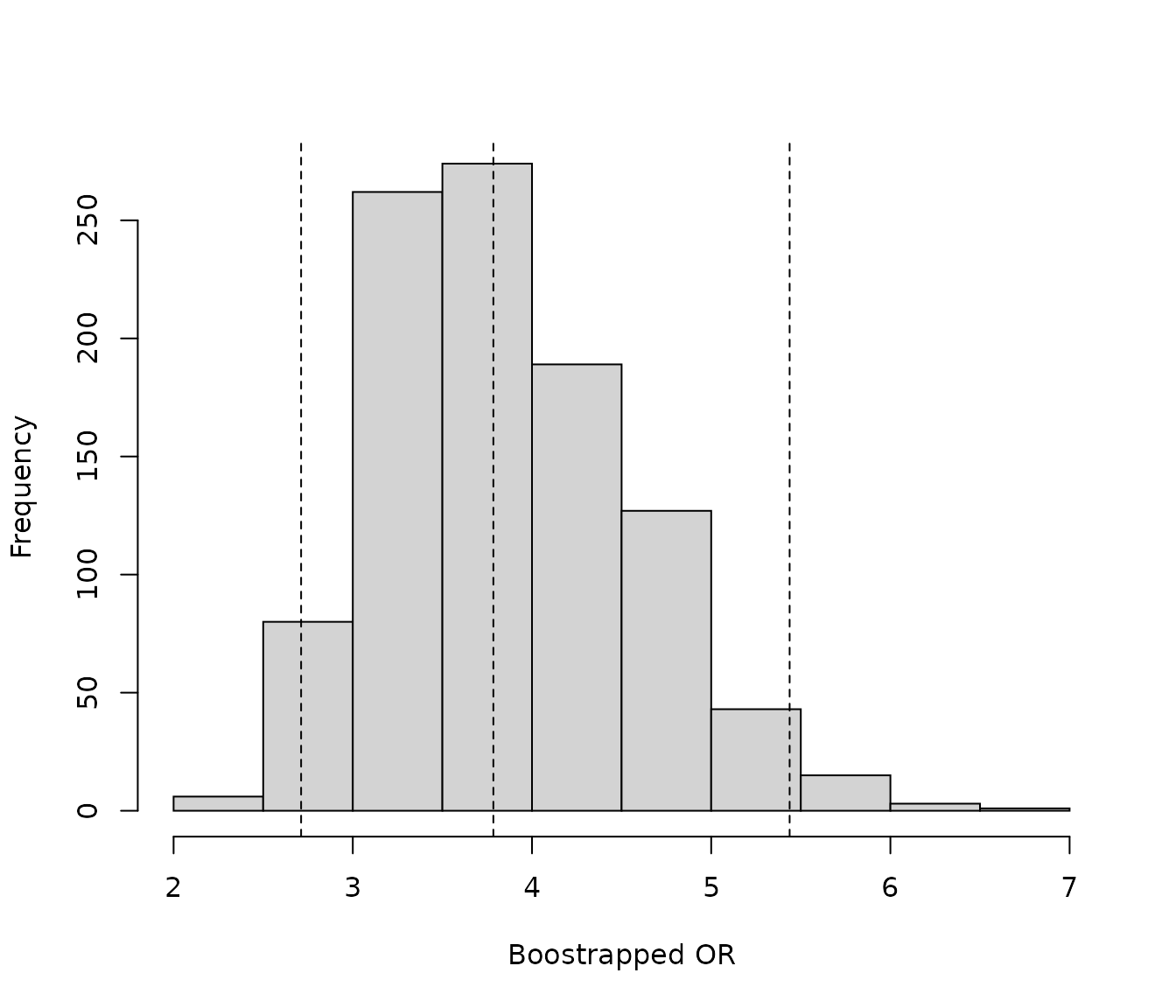
To test the distribution of the bootstrapped HRs, a histogram can be plotted. If the plot does not appear normally distributed, this may suggest that the BCa approach is more appropriate than the percentile approach.

# Summarize bootstrap estimates in a histogram
# Vertical lines indicate the median and upper and lower CIs
hist(HR_bootstraps$t, main = "", xlab = "Boostrapped HR")
abline(v= quantile(HR_bootstraps$t, probs = c(0.025, 0.5, 0.975)), lty=2)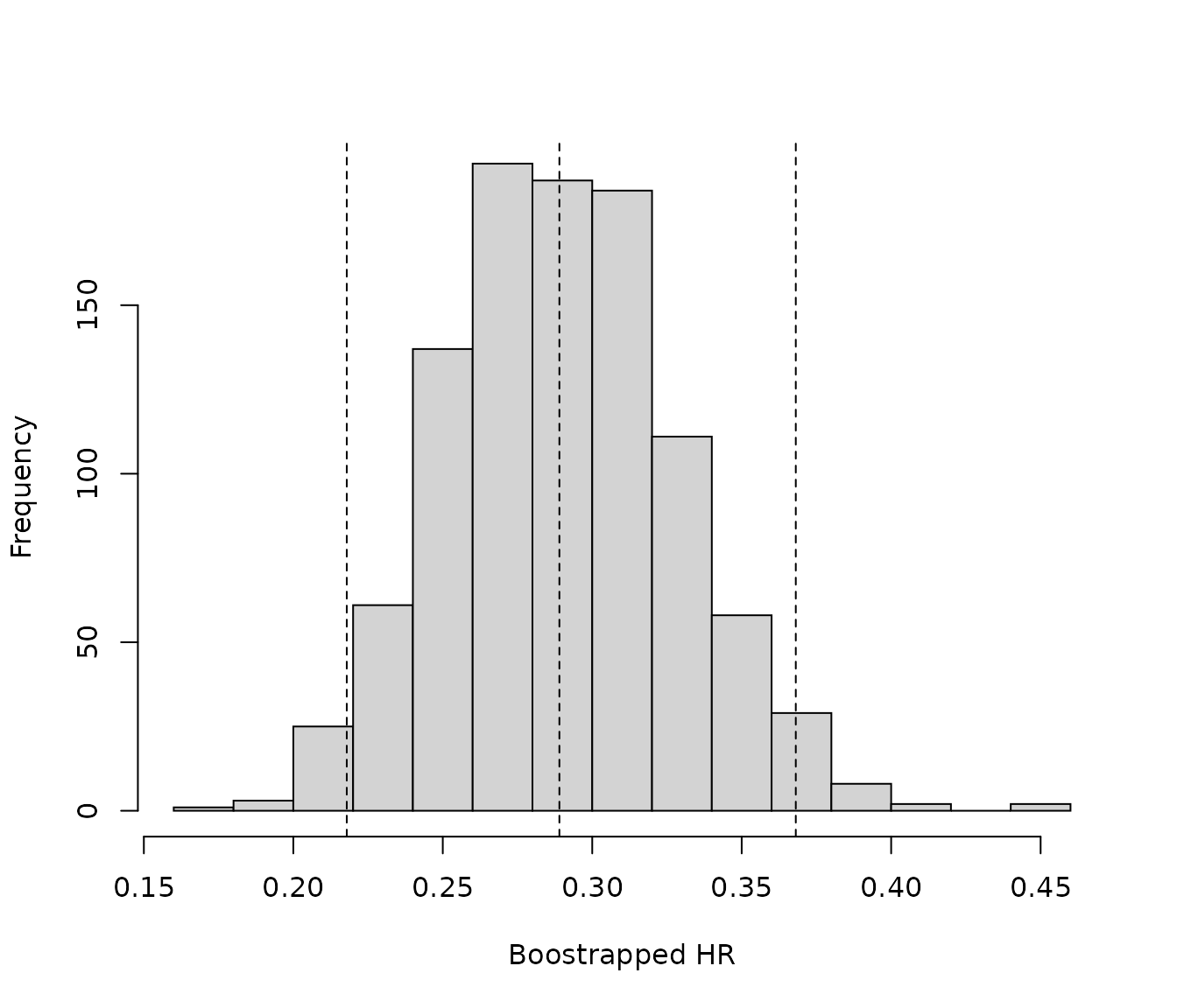

Example for response data

Estimating the odds ratio (OR)

In this example, the weighted OR 3.79 (95% CI: 2.56, 5.60) shows a smaller treatment effect (closer to 1) than the unweighted OR 5.32 (95% CI: 3.89, 7.28) indicating a smaller difference between treatments. The median of the bootstrap OR samples was similar to the OR from the weighted logistic regression model to two decimal places. The median OR from the bootstrap samples was 3.78 compared with the OR of 3.79 from the weighted logistic regression model. For this endpoint, the percentile CI (2.69 to 5.44) and BCa confidence interval (2.67, 5.40) are similar, suggesting the bootstrap samples are relatively normally distributed (see diagnostics). Finally, it should be noted that results are relatively consistent across all methods, the intervention treatment significantly increases the odds of response compared with the comparator treatment.

When deriving the weighted OR using the GLM, the warnings have been suppressed, since the function expects integer values for response (i.e. 1 or 0) however, when the weights function is used, the response values are no longer a integer value.

## Calculate ORs

# Fit a logistic regression model without weights to estimate the unweighted OR
unweighted_OR <- glm(formula = response~ARM,
                     family = binomial(link="logit"),
                     data = combined_data)

# Log odds ratio
log_OR_CI_logit <- cbind(coef(unweighted_OR), confint.default(unweighted_OR, level = 0.95))[2,]

# Odds ratio
OR_CI_logit <- exp(log_OR_CI_logit)
#tidy up naming
names(OR_CI_logit) <- c("OR", "OR_low_CI", "OR_upp_CI")

# Fit a logistic regression model with weights to estimate the weighted OR
weighted_OR <- suppressWarnings(glm(formula = response~ARM,
                                    family = binomial(link="logit"),
                                    data = combined_data,
                                    weight = wt))

# Weighted log odds ratio
log_OR_CI_logit_wtd <- cbind(coef(weighted_OR), confint.default(weighted_OR, level = 0.95))[2,]

# Weighted odds ratio
OR_CI_logit_wtd <- exp(log_OR_CI_logit_wtd)
#tidy up naming
names(OR_CI_logit_wtd) <- c("OR", "OR_low_CI", "OR_upp_CI")

OR_CI_logit_wtd
#>        OR OR_low_CI OR_upp_CI 
#>  3.786515  2.558141  5.604732

## Bootstrapping

# Bootstrap 1000 ORs
OR_bootstraps <- boot(data = est_weights$analysis_data, # intervention data
                      statistic = bootstrap_OR, # bootstrap the OR
                      R = 1000, # number of bootstrap samples
                      comparator_data = comparator_input, # comparator pseudo data
                      matching = est_weights$matching_vars, # matching variables
                      model = 'response ~ ARM' # model to fit
                      )


# Median of the bootstrap samples
OR_median <- median(OR_bootstraps$t)

# Bootstrap CI - Percentile CI
boot_ci_OR <- boot.ci(boot.out = OR_bootstraps, index=1, type="perc")

# Bootstrap CI - BCa CI
boot_ci_OR_BCA <- boot.ci(boot.out = OR_bootstraps, index=1, type="bca")


## Summary

# Produce summary of ORs and CIs
OR_summ <- rbind(OR_CI_logit, OR_CI_logit_wtd) %>% # Unweighted and weighted ORs and CIs
  as.data.frame() %>%
  mutate(Method = c("OR (95% CI) from unadjusted logistic regression model",
                    "OR (95% CI) from weighted logistic regression model")) %>%

  # Median bootstrapped HR and 95% percentile CI
  rbind(data.frame("OR" = OR_median,
                   "OR_low_CI" = boot_ci_OR$percent[4],
                   "OR_upp_CI" = boot_ci_OR$percent[5],
                   "Method"="Bootstrap median HR (95% percentile CI)")) %>%

  # Median bootstrapped HR and 95% bias-corrected and accelerated bootstrap CI
  rbind(data.frame("OR" = OR_median,
                   "OR_low_CI" = boot_ci_OR_BCA$bca[4],
                   "OR_upp_CI" = boot_ci_OR_BCA$bca[5],
                   "Method"="Bootstrap median HR (95% BCa CI)")) %>%
  #apply rounding for numeric columns
  mutate_if(.predicate = is.numeric, sprintf, fmt = "%.3f") %>%
  #format for output
  transmute(Method, OR_95_CI = paste0(OR, " (", OR_low_CI, " to ", OR_upp_CI, ")"))

# turns the results to a table suitable for word/ powerpoint
OR_table <- OR_summ %>%
  regulartable() %>% #make it a flextable object
  set_header_labels(Method = "Method",  OR_95_CI = "Odds ratio (95% CI)")  %>%
  font(font = 'Arial', part = 'all') %>%
  fontsize(size = 14, part = 'all') %>%
  bold(part = 'header') %>%
  align(align = 'center', part = 'all') %>%
  align(j = 1, align = 'left', part = 'all') %>%
  border_outer(border = fp_border()) %>%
  border_inner_h(border = fp_border()) %>%
  border_inner_v(border = fp_border()) %>%
  autofit(add_w = 0.2)
OR_table

Method	Odds ratio (95% CI)
OR (95% CI) from unadjusted logistic regression model	5.318 (3.888 to 7.275)
OR (95% CI) from weighted logistic regression model	3.787 (2.558 to 5.605)
Bootstrap median HR (95% percentile CI)	3.784 (2.693 to 5.448)
Bootstrap median HR (95% BCa CI)	3.784 (2.669 to 5.402)

Bootstrapping diagnostics

To test the distribution of the bootstrapped ORs, a histogram can be plotted. If the plot does not appear normally distributed, this may suggest that the BCa approach is more appropriate than the percentile approach.

# Summarize bootstrap estimates in a histogram
# Vertical lines indicate the median and upper and lower CIs
hist(OR_bootstraps$t, main = "", xlab = "Boostrapped OR")
abline(v= quantile(OR_bootstraps$t, probs = c(0.025,0.5,0.975)), lty=2)

References

[1]

Signorovitch JE, Sikirica V, Erder MH, Xie J, Lu M, Hodgkins PS, et al. Matching-adjusted indirect comparisons: A new tool for timely comparative effectiveness research. Value in Health 2012;15:940–7.

[2]

Phillippo D, Ades T, Dias S, Palmer S, Abrams KR, Welton N. NICE DSU technical support document 18: Methods for population-adjusted indirect comparisons in submissions to NICE 2016.

[3]

Phillippo DM, Dias S, Elsada A, Ades A, Welton NJ. Population adjustment methods for indirect comparisons: A review of national institute for health and care excellence technology appraisals. International Journal of Technology Assessment in Health Care 2019;35:221–8.

[4]

Guyot P, Ades A, Ouwens MJ, Welton NJ. Enhanced secondary analysis of survival data: Reconstructing the data from published kaplan-meier survival curves. BMC Medical Research Methodology 2012;12:9.

[5]

Austin PC. Variance estimation when using inverse probability of treatment weighting (IPTW) with survival analysis. Statistics in Medicine 2016;35:5642–55.

[6]

Therneau TM, Crowson CS, Atkinson EJ. Adjusted survival curves. 2015.

[7]

Efron B, Tibshirani RJ. An introduction to the bootstrap. CRC press; 1994.

[8]

DiCiccio TJ, Efron B. Bootstrap confidence intervals. Statistical Science 1996:189–212.

[9]

Efron B. Better bootstrap confidence intervals. Journal of the American Statistical Association 1987;82:171–85.

Matching-Adjusted Indirect Comparison: Example using the `MAIC` package

Roche

2022-07-26

Introduction

Example Scenario

Set up packages and data

Install packages

Read in the data

Intervention trial IPD

Baseline data from the comparator trial

Estimate weights

Statistical theory

Optimization procedure

Weight diagnostics

Are the weights sensible?

Effective sample size

Rescaled weights

Overall weight diagnostics summary function

Has the optimization worked?

Incorporation of the weights in statistical analysis

Comparator pseudo data

Estimating the relative effect

Bootstrapping a confidence interval

Example for survival data

Kaplan-Meier plot

Estimating the hazard ratio (HR)

Bootstrapping diagnostics

Example for response data

Estimating the odds ratio (OR)

Bootstrapping diagnostics

References

Matching-Adjusted Indirect Comparison: Example using the MAIC package

Roche

2022-07-26

Introduction

Example Scenario

Set up packages and data

Install packages

Read in the data

Intervention trial IPD

Baseline data from the comparator trial

Estimate weights

Statistical theory

Optimization procedure

Weight diagnostics

Are the weights sensible?

Effective sample size

Rescaled weights

Overall weight diagnostics summary function

Has the optimization worked?

Incorporation of the weights in statistical analysis

Comparator pseudo data

Estimating the relative effect

Bootstrapping a confidence interval

Example for survival data

Kaplan-Meier plot

Estimating the hazard ratio (HR)

Bootstrapping diagnostics

Example for response data

Estimating the odds ratio (OR)

Bootstrapping diagnostics

References

Matching-Adjusted Indirect Comparison: Example using the `MAIC` package