Estimate effective sample size
estimate_ess.RdEstimate the effective sample size (ESS).
estimate_ess(data, wt_col = "wt")Arguments
- data
A data frame containing individual patient data from the intervention study, including a column containing the weights (derived using
estimate_weights).- wt_col
The name of the weights column in the data frame containing the intervention individual patient data and the MAIC propensity weights. The default is wt.
Value
The effective sample size (ESS) as a numeric value.
Details
For a weighted estimate, the effective sample size (ESS) is the number of independent non-weighted individuals that would be required to give an estimate with the same precision as the weighted sample estimate. A small ESS, relative to the original sample size, is an indication that the weights are highly variable and that the estimate may be unstable. This often occurs if there is very limited overlap in the distribution of the matching variables between the populations being compared. If there is insufficient overlap between populations it may not be possible to obtain reliable estimates of the weights
References
NICE DSU TECHNICAL SUPPORT DOCUMENT 18: METHODS FOR POPULATION-ADJUSTED INDIRECT COMPARISONS IN SUBMSISSIONS TO NICE, REPORT BY THE DECISION SUPPORT UNIT, December 2016
See also
Examples
# This example code uses the weighted individual patient data, outputted from
# the estimate_weights function to perform weight diagnostics. The weighted data
# is saved within est_weights. To check the weighted aggregate baseline
# characteristics for 'intervention' match those in the comparator data,
# standardized data "target_pop_standard" is used. Please see the package
# vignette for more information on how to use the estimate_weights function and
# derive the "target_pop_standard" data.
library(dplyr)
library(MAIC)
# load est_weights
data(est_weights, package = "MAIC")
# load target_pop_standard
data(target_pop_standard, package = "MAIC")
# List out the uncentered variables used in the matching
match_cov <- c("AGE",
"SEX",
"SMOKE",
"ECOG0")
# Are the weights sensible? ----------------------------------------------------
# The wt_diagnostics function requires the output from the estimate_weights
# function and will output:
# - the effective sample size (ESS)
# - a summary of the weights and rescaled weights (mean, standard deviation,
# median, minimum and maximum)
# - a unique set of weights with the corresponding patient profile based on the
# matching variables
diagnostics <- wt_diagnostics(est_weights$analysis_data,
vars = match_cov)
diagnostics$ESS
#> [1] 157.0715
diagnostics$Summary_of_weights
#> type mean sd median min max
#> 1 Weights 0.3763805 0.556692 0.03467630 1.855194e-11 2.373310
#> 2 Rescaled weights 1.0000000 1.479067 0.09213098 4.929037e-11 6.305614
diagnostics$Weight_profiles
#> AGE SEX SMOKE ECOG0 wt wt_rs
#> 1 45 1 0 0 1.301506e+00 3.457953e+00
#> 2 71 1 0 0 7.024764e-08 1.866400e-07
#> 3 58 1 1 1 6.384284e-02 1.696231e-01
#> 4 48 0 0 1 1.204094e+00 3.199141e+00
#> 5 69 1 0 1 1.371621e-06 3.644239e-06
#> 6 47 1 1 0 1.010290e+00 2.684226e+00
#> 7 61 1 1 0 7.016834e-03 1.864293e-02
#> 8 54 0 1 1 2.610269e-01 6.935186e-01
#> 9 56 0 1 0 1.165019e-01 3.095323e-01
#> 10 63 0 0 0 1.212450e-03 3.221341e-03
#> 11 50 0 0 0 1.277640e+00 3.394543e+00
#> 12 57 1 0 1 2.355647e-01 6.258685e-01
#> 13 62 0 1 1 1.515077e-03 4.025386e-03
#> 14 57 0 0 1 1.307047e-01 3.472675e-01
#> 15 66 1 0 0 7.757577e-05 2.061100e-04
#> 16 75 1 1 1 3.343552e-11 8.883437e-11
#> 17 47 0 0 0 1.126587e+00 2.993213e+00
#> 18 57 1 0 0 2.470419e-01 6.563622e-01
#> 19 54 1 0 0 9.915215e-01 2.634359e+00
#> 20 55 1 1 0 3.336792e-01 8.865476e-01
#> 21 64 1 0 1 7.360573e-04 1.955620e-03
#> 22 53 0 1 0 3.765647e-01 1.000489e+00
#> 23 47 1 0 0 2.030410e+00 5.394567e+00
#> 24 60 0 1 0 8.875806e-03 2.358200e-02
#> 25 49 0 0 1 1.255669e+00 3.336168e+00
#> 26 55 0 0 0 3.720898e-01 9.886001e-01
#> 27 66 0 0 1 4.104372e-05 1.090485e-04
#> 28 58 1 0 1 1.283068e-01 3.408965e-01
#> 29 49 1 0 1 2.263049e+00 6.012663e+00
#> 30 61 1 0 0 1.410194e-02 3.746723e-02
#> 31 66 1 1 0 3.860012e-05 1.025561e-04
#> 32 59 0 1 1 1.795110e-02 4.769403e-02
#> 33 74 0 1 0 1.218200e-10 3.236619e-10
#> 34 73 0 0 0 1.426210e-09 3.789276e-09
#> 35 74 1 0 1 4.207407e-10 1.117860e-09
#> 36 58 0 1 1 3.542365e-02 9.411659e-02
#> 37 61 0 0 1 7.461039e-03 1.982313e-02
#> 38 47 0 1 1 5.345235e-01 1.420168e+00
#> 39 73 0 1 1 6.766831e-10 1.797870e-09
#> 40 68 1 0 0 5.841352e-06 1.551981e-05
#> 41 49 0 0 0 1.316848e+00 3.498714e+00
#> 42 71 0 0 0 3.897740e-08 1.035585e-07
#> 43 70 1 0 1 3.142487e-07 8.349228e-07
#> 44 62 0 1 0 1.588895e-03 4.221512e-03
#> 45 49 1 0 0 2.373310e+00 6.305614e+00
#> 46 74 0 0 0 2.448252e-10 6.504727e-10
#> 47 46 0 0 1 8.916746e-01 2.369078e+00
#> 48 68 0 1 0 1.612713e-06 4.284793e-06
#> 49 46 1 1 0 8.385873e-01 2.228031e+00
#> 50 75 0 1 1 1.855194e-11 4.929037e-11
#> 51 56 1 0 1 4.023732e-01 1.069060e+00
#> 52 72 0 0 0 7.729812e-09 2.053723e-08
#> 53 57 1 1 1 1.172122e-01 3.114193e-01
#> 54 46 1 0 0 1.685333e+00 4.477738e+00
#> 55 56 0 1 1 1.110894e-01 2.951518e-01
#> 56 73 1 0 1 2.450991e-09 6.512004e-09
#> 57 60 0 1 1 8.463447e-03 2.248641e-02
#> 58 75 1 0 0 7.047030e-11 1.872316e-10
#> 59 69 0 1 1 3.786845e-07 1.006122e-06
#> 60 47 0 0 1 1.074247e+00 2.854152e+00
#> 61 74 1 0 0 4.412402e-10 1.172325e-09
#> 62 71 0 0 1 3.716656e-08 9.874729e-08
#> 63 49 0 1 1 6.247950e-01 1.660009e+00
#> 64 45 0 0 0 7.221499e-01 1.918670e+00
#> 65 68 0 0 0 3.241115e-06 8.611273e-06
#> 66 60 1 0 0 3.214876e-02 8.541558e-02
#> 67 45 0 1 0 3.593270e-01 9.546908e-01
#> 68 57 0 0 0 1.370730e-01 3.641872e-01
#> 69 50 0 0 1 1.218282e+00 3.236837e+00
#> 70 63 1 0 1 2.083637e-03 5.535987e-03
#> 71 68 0 0 1 3.090537e-06 8.211204e-06
#> 72 51 1 0 0 2.078541e+00 5.522446e+00
#> 73 52 0 1 0 4.819386e-01 1.280456e+00
#> 74 69 1 1 1 6.824903e-07 1.813299e-06
#> 75 70 0 0 1 1.743631e-07 4.632628e-07
#> 76 72 1 0 0 1.393118e-08 3.701355e-08
#> 77 51 1 1 0 1.034239e+00 2.747856e+00
#> 78 69 0 0 1 7.610533e-07 2.022032e-06
#> 79 73 0 1 0 7.096527e-10 1.885466e-09
#> 80 62 0 0 1 3.044894e-03 8.089934e-03
#> 81 67 1 1 0 1.098128e-05 2.917601e-05
#> 82 54 0 1 0 2.737447e-01 7.273085e-01
#> 83 52 0 1 1 4.595483e-01 1.220967e+00
#> 84 57 0 1 1 6.503599e-02 1.727932e-01
#> 85 67 0 1 1 5.809967e-06 1.543642e-05
#> 86 74 0 1 1 1.161604e-10 3.086249e-10
#> 87 72 0 1 0 3.846196e-09 1.021890e-08
#> 88 69 0 1 0 3.971349e-07 1.055142e-06
#> 89 55 1 0 0 6.706048e-01 1.781720e+00
#> 90 53 1 0 0 1.363942e+00 3.623839e+00
#> 91 69 1 0 0 1.438449e-06 3.821795e-06
#> 92 68 1 0 1 5.569970e-06 1.479877e-05
#> 93 58 1 0 0 1.345582e-01 3.575058e-01
#> 94 64 0 0 0 4.283051e-04 1.137958e-03
#> 95 64 0 1 0 2.131159e-04 5.662245e-04
#> 96 64 1 1 0 3.840915e-04 1.020487e-03
#> 97 55 1 0 1 6.394493e-01 1.698944e+00
#> 98 50 1 0 1 2.195669e+00 5.833641e+00
#> 99 59 0 0 0 3.783460e-02 1.005222e-01
#> 100 71 0 1 0 1.939435e-08 5.152859e-08
#> 101 56 0 0 1 2.232596e-01 5.931752e-01
#> 102 51 1 0 1 1.981974e+00 5.265879e+00
#> 103 65 1 0 1 2.419131e-04 6.427356e-04
#> 104 45 1 1 1 6.175160e-01 1.640669e+00
#> 105 71 0 1 1 1.849332e-08 4.913463e-08
#> 106 65 1 0 0 2.536997e-04 6.740512e-04
#> 107 67 0 0 0 1.224536e-05 3.253453e-05
#> 108 48 0 0 0 1.262761e+00 3.355011e+00
#> 109 53 1 1 1 6.471395e-01 1.719376e+00
#> 110 70 0 1 1 8.675950e-08 2.305101e-07
#> 111 54 0 0 0 5.501527e-01 1.461693e+00
#> 112 58 0 0 0 7.466057e-02 1.983646e-01
#> 113 59 0 0 1 3.607685e-02 9.585207e-02
#> 114 75 0 0 1 3.728436e-11 9.906029e-11
#> 115 48 1 1 0 1.132407e+00 3.008675e+00
#> 116 63 0 0 1 1.156121e-03 3.071681e-03
#> 117 53 0 0 0 7.567929e-01 2.010712e+00
#> 118 75 0 1 0 1.945583e-11 5.169192e-11
#> 119 45 0 1 1 3.426331e-01 9.103370e-01
#> 120 53 0 1 1 3.590699e-01 9.540078e-01
#> 121 52 0 0 1 9.235676e-01 2.453814e+00
#> 122 61 0 1 0 3.893340e-03 1.034416e-02
#> 123 70 1 0 0 3.295596e-07 8.756022e-07
#> 124 52 1 0 0 1.745614e+00 4.637896e+00
#> 125 55 0 1 0 1.851443e-01 4.919072e-01
#> 126 57 0 1 0 6.820470e-02 1.812121e-01
#> 127 49 0 1 0 6.552365e-01 1.740889e+00
#> 128 61 0 0 0 7.824558e-03 2.078896e-02
#> 129 51 0 0 0 1.153293e+00 3.064168e+00
#> 130 59 0 1 0 1.882572e-02 5.001779e-02
#> 131 59 1 1 1 3.235266e-02 8.595733e-02
#> 132 58 0 1 0 3.714957e-02 9.870217e-02
#> 133 67 1 0 0 2.206940e-05 5.863588e-05
#> 134 51 0 1 0 5.738550e-01 1.524667e+00
#> 135 68 1 1 1 2.771503e-06 7.363567e-06
#> 136 61 1 0 1 1.344678e-02 3.572655e-02
#> 137 52 1 1 0 8.685815e-01 2.307722e+00
#> 138 51 1 1 1 9.861898e-01 2.620194e+00
#> 139 60 0 0 0 1.783797e-02 4.739344e-02
#> 140 71 1 0 1 6.698402e-08 1.779689e-07
#> 141 56 0 0 0 2.341373e-01 6.220761e-01
#> 142 74 1 1 0 2.195521e-10 5.833248e-10
#> 143 66 0 0 0 4.304346e-05 1.143616e-04
#> 144 70 0 1 0 9.098662e-08 2.417411e-07
#> 145 47 0 1 0 5.605667e-01 1.489362e+00
#> 146 54 0 0 1 5.245933e-01 1.393784e+00
#> 147 65 0 0 1 1.342272e-04 3.566264e-04
#> 148 47 1 0 1 1.936079e+00 5.143942e+00
#> 149 50 1 0 0 2.302647e+00 6.117870e+00
#> 150 67 0 1 0 6.093042e-06 1.618852e-05
#> 151 72 1 1 0 6.931869e-09 1.841718e-08
#> 152 45 0 0 1 6.885997e-01 1.829531e+00
#> 153 60 0 0 1 1.700924e-02 4.519160e-02
#> 154 58 0 0 1 7.119193e-02 1.891488e-01
#> 155 69 1 1 0 7.157428e-07 1.901647e-06
#> 156 66 0 1 1 2.042251e-05 5.426029e-05
#> 157 73 1 0 0 2.570409e-09 6.829284e-09
#> 158 55 0 1 1 1.765427e-01 4.690538e-01
#> 159 66 1 0 1 7.397170e-05 1.965344e-04
#> 160 63 1 0 0 2.185157e-03 5.805713e-03
#> 161 53 1 0 1 1.300575e+00 3.455479e+00
#> 162 59 1 0 0 6.818802e-02 1.811678e-01
#> 163 75 0 0 0 3.910094e-11 1.038867e-10
#> 164 54 1 0 1 9.454567e-01 2.511970e+00
#> 165 62 0 0 0 3.193248e-03 8.484095e-03
#> 166 54 1 1 0 4.933608e-01 1.310803e+00
#> 167 55 0 0 1 3.548030e-01 9.426710e-01
#> 168 69 0 0 0 7.981336e-07 2.120550e-06
#> 169 48 0 1 1 5.991327e-01 1.591827e+00
#> 170 74 0 0 1 2.334509e-10 6.202525e-10
#> 171 62 1 0 0 5.755082e-03 1.529060e-02
#> 172 52 0 0 0 9.685659e-01 2.573369e+00
#> 173 51 0 1 1 5.471944e-01 1.453833e+00
#> 174 56 1 0 0 4.219777e-01 1.121147e+00
#> 175 57 1 1 0 1.229230e-01 3.265924e-01
#> 176 65 0 0 0 1.407671e-04 3.740020e-04
#> 177 67 0 0 1 1.167646e-05 3.102302e-05
#> 178 53 0 0 1 7.216332e-01 1.917297e+00
#> 179 46 0 0 0 9.351191e-01 2.484505e+00
#> 180 65 0 1 1 6.678871e-05 1.774500e-04
#> 181 72 0 1 1 3.667507e-09 9.744146e-09
#> 182 60 1 1 1 1.525338e-02 4.052650e-02
#> 183 59 1 0 1 6.502008e-02 1.727509e-01
#> 184 46 0 1 0 4.652961e-01 1.236239e+00
#> 185 70 1 1 1 1.563637e-07 4.154405e-07
#> 186 50 0 1 1 6.061923e-01 1.610584e+00
#> 187 68 0 1 1 1.537788e-06 4.085727e-06
#> 188 48 1 0 0 2.275831e+00 6.046622e+00
#> 189 75 1 1 0 3.506458e-11 9.316259e-11
#> 190 50 0 1 0 6.357274e-01 1.689055e+00
#> 191 75 1 0 1 6.719634e-11 1.785330e-10
#> 192 59 1 1 0 3.392896e-02 9.014537e-02
#> 193 48 0 1 0 6.283238e-01 1.669385e+00
#> 194 62 1 0 1 5.487708e-03 1.458021e-02
#> 195 70 0 0 0 1.828585e-07 4.858340e-07
#> 196 56 1 1 0 2.099675e-01 5.578596e-01
#> 197 46 0 1 1 4.436790e-01 1.178804e+00
#> 198 67 1 1 1 1.047111e-05 2.782053e-05
# Each of the wt_diagnostics outputs can also be estimated individually
ESS <- estimate_ess(est_weights$analysis_data)
weight_summ <- summarize_wts(est_weights$analysis_data)
wts_profile <- profile_wts(est_weights$analysis_data, vars = match_cov)
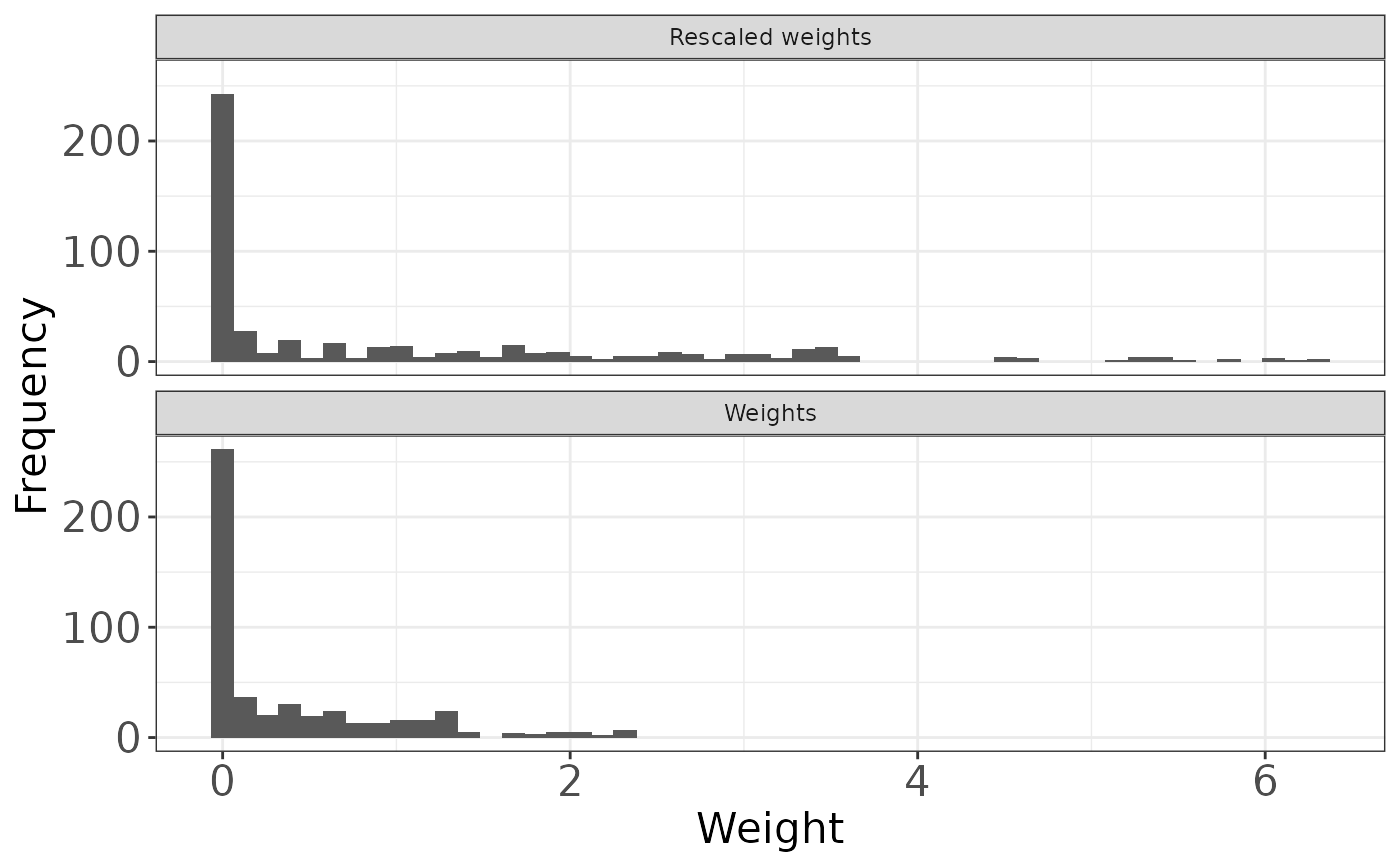
# Plot histograms of unscaled and rescaled weights
# bin_width needs to be adapted depending on the sample size in the data set
histogram <- hist_wts(est_weights$analysis_data, bin = 50)
histogram
 # Has the optimization worked? -------------------------------------------------
# The following code produces a summary table of the intervention baseline
# characteristics before and after matching compared with the comparator
# baseline characteristics:
# Create an object to hold the output
baseline_summary <- list('Intervention' = NA,
'Intervention_weighted' = NA,
'Comparator' = NA)
# Summarise matching variables for weighted intervention data
baseline_summary$Intervention_weighted <- est_weights$analysis_data %>%
transmute(AGE, SEX, SMOKE, ECOG0, wt) %>%
summarise_at(match_cov, list(~ weighted.mean(., wt)))
# Summarise matching variables for unweighted intervention data
baseline_summary$Intervention <- est_weights$analysis_data %>%
transmute(AGE, SEX, SMOKE, ECOG0, wt) %>%
summarise_at(match_cov, list(~ mean(.)))
# baseline data for the comparator study
baseline_summary$Comparator <- transmute(target_pop_standard,
AGE,
SEX,
SMOKE,
ECOG0)
# Combine the three summaries
# Takes a list of data frames and binds these together
trt <- names(baseline_summary)
baseline_summary <- bind_rows(baseline_summary) %>%
transmute_all(sprintf, fmt = "%.2f") %>% #apply rounding for presentation
transmute(ARM = as.character(trt), AGE, SEX, SMOKE, ECOG0)
# Insert N of intervention as number of patients
baseline_summary$`N/ESS`[baseline_summary$ARM == "Intervention"] <- nrow(est_weights$analysis_data)
# Insert N for comparator from target_pop_standard
baseline_summary$`N/ESS`[baseline_summary$ARM == "Comparator"] <- target_pop_standard$N
# Insert the ESS as the sample size for the weighted data
# This is calculated above but can also be obtained using the estimate_ess function as shown below
baseline_summary$`N/ESS`[baseline_summary$ARM == "Intervention_weighted"] <- est_weights$analysis_data %>%
estimate_ess(wt_col = 'wt')
baseline_summary <- baseline_summary %>%
transmute(ARM, `N/ESS`=round(`N/ESS`,1), AGE, SEX, SMOKE, ECOG0)
# Has the optimization worked? -------------------------------------------------
# The following code produces a summary table of the intervention baseline
# characteristics before and after matching compared with the comparator
# baseline characteristics:
# Create an object to hold the output
baseline_summary <- list('Intervention' = NA,
'Intervention_weighted' = NA,
'Comparator' = NA)
# Summarise matching variables for weighted intervention data
baseline_summary$Intervention_weighted <- est_weights$analysis_data %>%
transmute(AGE, SEX, SMOKE, ECOG0, wt) %>%
summarise_at(match_cov, list(~ weighted.mean(., wt)))
# Summarise matching variables for unweighted intervention data
baseline_summary$Intervention <- est_weights$analysis_data %>%
transmute(AGE, SEX, SMOKE, ECOG0, wt) %>%
summarise_at(match_cov, list(~ mean(.)))
# baseline data for the comparator study
baseline_summary$Comparator <- transmute(target_pop_standard,
AGE,
SEX,
SMOKE,
ECOG0)
# Combine the three summaries
# Takes a list of data frames and binds these together
trt <- names(baseline_summary)
baseline_summary <- bind_rows(baseline_summary) %>%
transmute_all(sprintf, fmt = "%.2f") %>% #apply rounding for presentation
transmute(ARM = as.character(trt), AGE, SEX, SMOKE, ECOG0)
# Insert N of intervention as number of patients
baseline_summary$`N/ESS`[baseline_summary$ARM == "Intervention"] <- nrow(est_weights$analysis_data)
# Insert N for comparator from target_pop_standard
baseline_summary$`N/ESS`[baseline_summary$ARM == "Comparator"] <- target_pop_standard$N
# Insert the ESS as the sample size for the weighted data
# This is calculated above but can also be obtained using the estimate_ess function as shown below
baseline_summary$`N/ESS`[baseline_summary$ARM == "Intervention_weighted"] <- est_weights$analysis_data %>%
estimate_ess(wt_col = 'wt')
baseline_summary <- baseline_summary %>%
transmute(ARM, `N/ESS`=round(`N/ESS`,1), AGE, SEX, SMOKE, ECOG0)