Weight diagnostics
wt_diagnostics.RdProduce a set of useful diagnostic metrics to summarize propensity weights
ESS (
estimate_ess)Summary statistics of the weights: minimum, maximum, median, mean, SD (
summarize_wts)Patient profile associated with weight values (
profile_wts)
wt_diagnostics(data, wt_col = "wt", wt_rs = "wt_rs", vars)Arguments
- data
A data frame containing individual patient data from the intervention study, including a column containing the weights (derived using estimate_weights).
- wt_col
The name of the weights column in the data frame containing the intervention individual patient data and the MAIC propensity weights. The default is wt.
- wt_rs
The name of the rescaled weights column in the data frame containing the intervention individual patient data and the MAIC propensity weights. The default is wt_rs.
- vars
A character vector giving the variable names of the baseline characteristics (not centered). These names must match the column names in the data.
Value
List of the following:
The effective sample size (ESS) as a numeric value.
A data frame that includes a summary (minimum, maximum, median, mean, standard deviation) of the weights and rescaled weights.
A data frame that includes a summary of patient characteristics associated with each weight value.
See also
Examples
# This example code uses the weighted individual patient data, outputted from
# the estimate_weights function to perform weight diagnostics. The weighted data
# is saved within est_weights. To check the weighted aggregate baseline
# characteristics for 'intervention' match those in the comparator data,
# standardized data "target_pop_standard" is used. Please see the package
# vignette for more information on how to use the estimate_weights function and
# derive the "target_pop_standard" data.
library(dplyr)
library(MAIC)
# load est_weights
data(est_weights, package = "MAIC")
# load target_pop_standard
data(target_pop_standard, package = "MAIC")
# List out the uncentered variables used in the matching
match_cov <- c("AGE",
"SEX",
"SMOKE",
"ECOG0")
# Are the weights sensible? ----------------------------------------------------
# The wt_diagnostics function requires the output from the estimate_weights
# function and will output:
# - the effective sample size (ESS)
# - a summary of the weights and rescaled weights (mean, standard deviation,
# median, minimum and maximum)
# - a unique set of weights with the corresponding patient profile based on the
# matching variables
diagnostics <- wt_diagnostics(est_weights$analysis_data,
vars = match_cov)
diagnostics$ESS
#> [1] 157.0715
diagnostics$Summary_of_weights
#> type mean sd median min max
#> 1 Weights 0.3763805 0.556692 0.03467630 1.855194e-11 2.373310
#> 2 Rescaled weights 1.0000000 1.479067 0.09213098 4.929037e-11 6.305614
diagnostics$Weight_profiles
#> AGE SEX SMOKE ECOG0 wt wt_rs
#> 1 45 1 0 0 1.301506e+00 3.457953e+00
#> 2 71 1 0 0 7.024764e-08 1.866400e-07
#> 3 58 1 1 1 6.384284e-02 1.696231e-01
#> 4 48 0 0 1 1.204094e+00 3.199141e+00
#> 5 69 1 0 1 1.371621e-06 3.644239e-06
#> 6 47 1 1 0 1.010290e+00 2.684226e+00
#> 7 61 1 1 0 7.016834e-03 1.864293e-02
#> 8 54 0 1 1 2.610269e-01 6.935186e-01
#> 9 56 0 1 0 1.165019e-01 3.095323e-01
#> 10 63 0 0 0 1.212450e-03 3.221341e-03
#> 11 50 0 0 0 1.277640e+00 3.394543e+00
#> 12 57 1 0 1 2.355647e-01 6.258685e-01
#> 13 62 0 1 1 1.515077e-03 4.025386e-03
#> 14 57 0 0 1 1.307047e-01 3.472675e-01
#> 15 66 1 0 0 7.757577e-05 2.061100e-04
#> 16 75 1 1 1 3.343552e-11 8.883437e-11
#> 17 47 0 0 0 1.126587e+00 2.993213e+00
#> 18 57 1 0 0 2.470419e-01 6.563622e-01
#> 19 54 1 0 0 9.915215e-01 2.634359e+00
#> 20 55 1 1 0 3.336792e-01 8.865476e-01
#> 21 64 1 0 1 7.360573e-04 1.955620e-03
#> 22 53 0 1 0 3.765647e-01 1.000489e+00
#> 23 47 1 0 0 2.030410e+00 5.394567e+00
#> 24 60 0 1 0 8.875806e-03 2.358200e-02
#> 25 49 0 0 1 1.255669e+00 3.336168e+00
#> 26 55 0 0 0 3.720898e-01 9.886001e-01
#> 27 66 0 0 1 4.104372e-05 1.090485e-04
#> 28 58 1 0 1 1.283068e-01 3.408965e-01
#> 29 49 1 0 1 2.263049e+00 6.012663e+00
#> 30 61 1 0 0 1.410194e-02 3.746723e-02
#> 31 66 1 1 0 3.860012e-05 1.025561e-04
#> 32 59 0 1 1 1.795110e-02 4.769403e-02
#> 33 74 0 1 0 1.218200e-10 3.236619e-10
#> 34 73 0 0 0 1.426210e-09 3.789276e-09
#> 35 74 1 0 1 4.207407e-10 1.117860e-09
#> 36 58 0 1 1 3.542365e-02 9.411659e-02
#> 37 61 0 0 1 7.461039e-03 1.982313e-02
#> 38 47 0 1 1 5.345235e-01 1.420168e+00
#> 39 73 0 1 1 6.766831e-10 1.797870e-09
#> 40 68 1 0 0 5.841352e-06 1.551981e-05
#> 41 49 0 0 0 1.316848e+00 3.498714e+00
#> 42 71 0 0 0 3.897740e-08 1.035585e-07
#> 43 70 1 0 1 3.142487e-07 8.349228e-07
#> 44 62 0 1 0 1.588895e-03 4.221512e-03
#> 45 49 1 0 0 2.373310e+00 6.305614e+00
#> 46 74 0 0 0 2.448252e-10 6.504727e-10
#> 47 46 0 0 1 8.916746e-01 2.369078e+00
#> 48 68 0 1 0 1.612713e-06 4.284793e-06
#> 49 46 1 1 0 8.385873e-01 2.228031e+00
#> 50 75 0 1 1 1.855194e-11 4.929037e-11
#> 51 56 1 0 1 4.023732e-01 1.069060e+00
#> 52 72 0 0 0 7.729812e-09 2.053723e-08
#> 53 57 1 1 1 1.172122e-01 3.114193e-01
#> 54 46 1 0 0 1.685333e+00 4.477738e+00
#> 55 56 0 1 1 1.110894e-01 2.951518e-01
#> 56 73 1 0 1 2.450991e-09 6.512004e-09
#> 57 60 0 1 1 8.463447e-03 2.248641e-02
#> 58 75 1 0 0 7.047030e-11 1.872316e-10
#> 59 69 0 1 1 3.786845e-07 1.006122e-06
#> 60 47 0 0 1 1.074247e+00 2.854152e+00
#> 61 74 1 0 0 4.412402e-10 1.172325e-09
#> 62 71 0 0 1 3.716656e-08 9.874729e-08
#> 63 49 0 1 1 6.247950e-01 1.660009e+00
#> 64 45 0 0 0 7.221499e-01 1.918670e+00
#> 65 68 0 0 0 3.241115e-06 8.611273e-06
#> 66 60 1 0 0 3.214876e-02 8.541558e-02
#> 67 45 0 1 0 3.593270e-01 9.546908e-01
#> 68 57 0 0 0 1.370730e-01 3.641872e-01
#> 69 50 0 0 1 1.218282e+00 3.236837e+00
#> 70 63 1 0 1 2.083637e-03 5.535987e-03
#> 71 68 0 0 1 3.090537e-06 8.211204e-06
#> 72 51 1 0 0 2.078541e+00 5.522446e+00
#> 73 52 0 1 0 4.819386e-01 1.280456e+00
#> 74 69 1 1 1 6.824903e-07 1.813299e-06
#> 75 70 0 0 1 1.743631e-07 4.632628e-07
#> 76 72 1 0 0 1.393118e-08 3.701355e-08
#> 77 51 1 1 0 1.034239e+00 2.747856e+00
#> 78 69 0 0 1 7.610533e-07 2.022032e-06
#> 79 73 0 1 0 7.096527e-10 1.885466e-09
#> 80 62 0 0 1 3.044894e-03 8.089934e-03
#> 81 67 1 1 0 1.098128e-05 2.917601e-05
#> 82 54 0 1 0 2.737447e-01 7.273085e-01
#> 83 52 0 1 1 4.595483e-01 1.220967e+00
#> 84 57 0 1 1 6.503599e-02 1.727932e-01
#> 85 67 0 1 1 5.809967e-06 1.543642e-05
#> 86 74 0 1 1 1.161604e-10 3.086249e-10
#> 87 72 0 1 0 3.846196e-09 1.021890e-08
#> 88 69 0 1 0 3.971349e-07 1.055142e-06
#> 89 55 1 0 0 6.706048e-01 1.781720e+00
#> 90 53 1 0 0 1.363942e+00 3.623839e+00
#> 91 69 1 0 0 1.438449e-06 3.821795e-06
#> 92 68 1 0 1 5.569970e-06 1.479877e-05
#> 93 58 1 0 0 1.345582e-01 3.575058e-01
#> 94 64 0 0 0 4.283051e-04 1.137958e-03
#> 95 64 0 1 0 2.131159e-04 5.662245e-04
#> 96 64 1 1 0 3.840915e-04 1.020487e-03
#> 97 55 1 0 1 6.394493e-01 1.698944e+00
#> 98 50 1 0 1 2.195669e+00 5.833641e+00
#> 99 59 0 0 0 3.783460e-02 1.005222e-01
#> 100 71 0 1 0 1.939435e-08 5.152859e-08
#> 101 56 0 0 1 2.232596e-01 5.931752e-01
#> 102 51 1 0 1 1.981974e+00 5.265879e+00
#> 103 65 1 0 1 2.419131e-04 6.427356e-04
#> 104 45 1 1 1 6.175160e-01 1.640669e+00
#> 105 71 0 1 1 1.849332e-08 4.913463e-08
#> 106 65 1 0 0 2.536997e-04 6.740512e-04
#> 107 67 0 0 0 1.224536e-05 3.253453e-05
#> 108 48 0 0 0 1.262761e+00 3.355011e+00
#> 109 53 1 1 1 6.471395e-01 1.719376e+00
#> 110 70 0 1 1 8.675950e-08 2.305101e-07
#> 111 54 0 0 0 5.501527e-01 1.461693e+00
#> 112 58 0 0 0 7.466057e-02 1.983646e-01
#> 113 59 0 0 1 3.607685e-02 9.585207e-02
#> 114 75 0 0 1 3.728436e-11 9.906029e-11
#> 115 48 1 1 0 1.132407e+00 3.008675e+00
#> 116 63 0 0 1 1.156121e-03 3.071681e-03
#> 117 53 0 0 0 7.567929e-01 2.010712e+00
#> 118 75 0 1 0 1.945583e-11 5.169192e-11
#> 119 45 0 1 1 3.426331e-01 9.103370e-01
#> 120 53 0 1 1 3.590699e-01 9.540078e-01
#> 121 52 0 0 1 9.235676e-01 2.453814e+00
#> 122 61 0 1 0 3.893340e-03 1.034416e-02
#> 123 70 1 0 0 3.295596e-07 8.756022e-07
#> 124 52 1 0 0 1.745614e+00 4.637896e+00
#> 125 55 0 1 0 1.851443e-01 4.919072e-01
#> 126 57 0 1 0 6.820470e-02 1.812121e-01
#> 127 49 0 1 0 6.552365e-01 1.740889e+00
#> 128 61 0 0 0 7.824558e-03 2.078896e-02
#> 129 51 0 0 0 1.153293e+00 3.064168e+00
#> 130 59 0 1 0 1.882572e-02 5.001779e-02
#> 131 59 1 1 1 3.235266e-02 8.595733e-02
#> 132 58 0 1 0 3.714957e-02 9.870217e-02
#> 133 67 1 0 0 2.206940e-05 5.863588e-05
#> 134 51 0 1 0 5.738550e-01 1.524667e+00
#> 135 68 1 1 1 2.771503e-06 7.363567e-06
#> 136 61 1 0 1 1.344678e-02 3.572655e-02
#> 137 52 1 1 0 8.685815e-01 2.307722e+00
#> 138 51 1 1 1 9.861898e-01 2.620194e+00
#> 139 60 0 0 0 1.783797e-02 4.739344e-02
#> 140 71 1 0 1 6.698402e-08 1.779689e-07
#> 141 56 0 0 0 2.341373e-01 6.220761e-01
#> 142 74 1 1 0 2.195521e-10 5.833248e-10
#> 143 66 0 0 0 4.304346e-05 1.143616e-04
#> 144 70 0 1 0 9.098662e-08 2.417411e-07
#> 145 47 0 1 0 5.605667e-01 1.489362e+00
#> 146 54 0 0 1 5.245933e-01 1.393784e+00
#> 147 65 0 0 1 1.342272e-04 3.566264e-04
#> 148 47 1 0 1 1.936079e+00 5.143942e+00
#> 149 50 1 0 0 2.302647e+00 6.117870e+00
#> 150 67 0 1 0 6.093042e-06 1.618852e-05
#> 151 72 1 1 0 6.931869e-09 1.841718e-08
#> 152 45 0 0 1 6.885997e-01 1.829531e+00
#> 153 60 0 0 1 1.700924e-02 4.519160e-02
#> 154 58 0 0 1 7.119193e-02 1.891488e-01
#> 155 69 1 1 0 7.157428e-07 1.901647e-06
#> 156 66 0 1 1 2.042251e-05 5.426029e-05
#> 157 73 1 0 0 2.570409e-09 6.829284e-09
#> 158 55 0 1 1 1.765427e-01 4.690538e-01
#> 159 66 1 0 1 7.397170e-05 1.965344e-04
#> 160 63 1 0 0 2.185157e-03 5.805713e-03
#> 161 53 1 0 1 1.300575e+00 3.455479e+00
#> 162 59 1 0 0 6.818802e-02 1.811678e-01
#> 163 75 0 0 0 3.910094e-11 1.038867e-10
#> 164 54 1 0 1 9.454567e-01 2.511970e+00
#> 165 62 0 0 0 3.193248e-03 8.484095e-03
#> 166 54 1 1 0 4.933608e-01 1.310803e+00
#> 167 55 0 0 1 3.548030e-01 9.426710e-01
#> 168 69 0 0 0 7.981336e-07 2.120550e-06
#> 169 48 0 1 1 5.991327e-01 1.591827e+00
#> 170 74 0 0 1 2.334509e-10 6.202525e-10
#> 171 62 1 0 0 5.755082e-03 1.529060e-02
#> 172 52 0 0 0 9.685659e-01 2.573369e+00
#> 173 51 0 1 1 5.471944e-01 1.453833e+00
#> 174 56 1 0 0 4.219777e-01 1.121147e+00
#> 175 57 1 1 0 1.229230e-01 3.265924e-01
#> 176 65 0 0 0 1.407671e-04 3.740020e-04
#> 177 67 0 0 1 1.167646e-05 3.102302e-05
#> 178 53 0 0 1 7.216332e-01 1.917297e+00
#> 179 46 0 0 0 9.351191e-01 2.484505e+00
#> 180 65 0 1 1 6.678871e-05 1.774500e-04
#> 181 72 0 1 1 3.667507e-09 9.744146e-09
#> 182 60 1 1 1 1.525338e-02 4.052650e-02
#> 183 59 1 0 1 6.502008e-02 1.727509e-01
#> 184 46 0 1 0 4.652961e-01 1.236239e+00
#> 185 70 1 1 1 1.563637e-07 4.154405e-07
#> 186 50 0 1 1 6.061923e-01 1.610584e+00
#> 187 68 0 1 1 1.537788e-06 4.085727e-06
#> 188 48 1 0 0 2.275831e+00 6.046622e+00
#> 189 75 1 1 0 3.506458e-11 9.316259e-11
#> 190 50 0 1 0 6.357274e-01 1.689055e+00
#> 191 75 1 0 1 6.719634e-11 1.785330e-10
#> 192 59 1 1 0 3.392896e-02 9.014537e-02
#> 193 48 0 1 0 6.283238e-01 1.669385e+00
#> 194 62 1 0 1 5.487708e-03 1.458021e-02
#> 195 70 0 0 0 1.828585e-07 4.858340e-07
#> 196 56 1 1 0 2.099675e-01 5.578596e-01
#> 197 46 0 1 1 4.436790e-01 1.178804e+00
#> 198 67 1 1 1 1.047111e-05 2.782053e-05
# Each of the wt_diagnostics outputs can also be estimated individually
ESS <- estimate_ess(est_weights$analysis_data)
weight_summ <- summarize_wts(est_weights$analysis_data)
wts_profile <- profile_wts(est_weights$analysis_data, vars = match_cov)
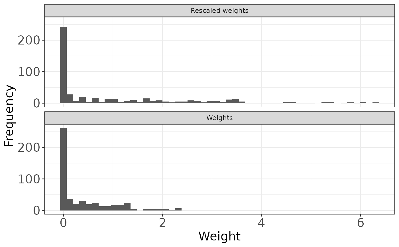
# Plot histograms of unscaled and rescaled weights
# bin_width needs to be adapted depending on the sample size in the data set
histogram <- hist_wts(est_weights$analysis_data, bin = 50)
histogram
 # Has the optimization worked? -------------------------------------------------
# The following code produces a summary table of the intervention baseline
# characteristics before and after matching compared with the comparator
# baseline characteristics:
# Create an object to hold the output
baseline_summary <- list('Intervention' = NA,
'Intervention_weighted' = NA,
'Comparator' = NA)
# Summarise matching variables for weighted intervention data
baseline_summary$Intervention_weighted <- est_weights$analysis_data %>%
transmute(AGE, SEX, SMOKE, ECOG0, wt) %>%
summarise_at(match_cov, list(~ weighted.mean(., wt)))
# Summarise matching variables for unweighted intervention data
baseline_summary$Intervention <- est_weights$analysis_data %>%
transmute(AGE, SEX, SMOKE, ECOG0, wt) %>%
summarise_at(match_cov, list(~ mean(.)))
# baseline data for the comparator study
baseline_summary$Comparator <- transmute(target_pop_standard,
AGE,
SEX,
SMOKE,
ECOG0)
# Combine the three summaries
# Takes a list of data frames and binds these together
trt <- names(baseline_summary)
baseline_summary <- bind_rows(baseline_summary) %>%
transmute_all(sprintf, fmt = "%.2f") %>% #apply rounding for presentation
transmute(ARM = as.character(trt), AGE, SEX, SMOKE, ECOG0)
# Insert N of intervention as number of patients
baseline_summary$`N/ESS`[baseline_summary$ARM == "Intervention"] <- nrow(est_weights$analysis_data)
# Insert N for comparator from target_pop_standard
baseline_summary$`N/ESS`[baseline_summary$ARM == "Comparator"] <- target_pop_standard$N
# Insert the ESS as the sample size for the weighted data
# This is calculated above but can also be obtained using the estimate_ess function as shown below
baseline_summary$`N/ESS`[baseline_summary$ARM == "Intervention_weighted"] <- est_weights$analysis_data %>%
estimate_ess(wt_col = 'wt')
baseline_summary <- baseline_summary %>%
transmute(ARM, `N/ESS`=round(`N/ESS`,1), AGE, SEX, SMOKE, ECOG0)
# Has the optimization worked? -------------------------------------------------
# The following code produces a summary table of the intervention baseline
# characteristics before and after matching compared with the comparator
# baseline characteristics:
# Create an object to hold the output
baseline_summary <- list('Intervention' = NA,
'Intervention_weighted' = NA,
'Comparator' = NA)
# Summarise matching variables for weighted intervention data
baseline_summary$Intervention_weighted <- est_weights$analysis_data %>%
transmute(AGE, SEX, SMOKE, ECOG0, wt) %>%
summarise_at(match_cov, list(~ weighted.mean(., wt)))
# Summarise matching variables for unweighted intervention data
baseline_summary$Intervention <- est_weights$analysis_data %>%
transmute(AGE, SEX, SMOKE, ECOG0, wt) %>%
summarise_at(match_cov, list(~ mean(.)))
# baseline data for the comparator study
baseline_summary$Comparator <- transmute(target_pop_standard,
AGE,
SEX,
SMOKE,
ECOG0)
# Combine the three summaries
# Takes a list of data frames and binds these together
trt <- names(baseline_summary)
baseline_summary <- bind_rows(baseline_summary) %>%
transmute_all(sprintf, fmt = "%.2f") %>% #apply rounding for presentation
transmute(ARM = as.character(trt), AGE, SEX, SMOKE, ECOG0)
# Insert N of intervention as number of patients
baseline_summary$`N/ESS`[baseline_summary$ARM == "Intervention"] <- nrow(est_weights$analysis_data)
# Insert N for comparator from target_pop_standard
baseline_summary$`N/ESS`[baseline_summary$ARM == "Comparator"] <- target_pop_standard$N
# Insert the ESS as the sample size for the weighted data
# This is calculated above but can also be obtained using the estimate_ess function as shown below
baseline_summary$`N/ESS`[baseline_summary$ARM == "Intervention_weighted"] <- est_weights$analysis_data %>%
estimate_ess(wt_col = 'wt')
baseline_summary <- baseline_summary %>%
transmute(ARM, `N/ESS`=round(`N/ESS`,1), AGE, SEX, SMOKE, ECOG0)