rpsftmPlus-vignette • rpsftmPlus

This vignette gives a short introduction to the R-package rpsftmPlus. The package implements useful functionalities to create sensible default plots and reports of analysis performed using the rpsftm package.

rpsftm.refit: rpsftm.refit(x, k). This function refits an rpsftm model varying the treat_modifier parameter. Allowing sensitivities to the common treatment effect assumption.
rpsftm.coxph: rpsftm.coxph(x). This function compares observed experimental and latent control arms with a cox model. It inflates the variance to account for the g-estimation step and correct the CI limits.
gg…: Various plotting functions for decriptive analysis, diagnostics and reporting.

Package installation

The package can be installed using the following commands in the R console.

# install package from github
devtools::install_github(
  'Roche/Global-HTA-Evidence-Open', subdir = "Rpackages/rpsftmPlus"
)

library(rpsftmPlus)
#> Loading required package: rpsftm
#> Warning: replacing previous import 'rpsftm::cox.zph' by 'survival::cox.zph' when
#> loading 'rpsftmPlus'
library(rpsftm)
library(survival)
#> 
#> Attaching package: 'survival'
#> The following object is masked from 'package:rpsftm':
#> 
#>     cox.zph
library(ggplot2)
library(dplyr)
#> 
#> Attaching package: 'dplyr'
#> The following objects are masked from 'package:stats':
#> 
#>     filter, lag
#> The following objects are masked from 'package:base':
#> 
#>     intersect, setdiff, setequal, union
library(reshape2)

We first need to derive time on experimental treatment and add to the data frame.

immdef <- rpsftm::immdef
immdef$rx <- with(immdef, 1 - xoyrs/progyrs)
pander::pander(immdef[1:5,])

id	def	imm	censyrs	xo	xoyrs	prog	progyrs	rx
1	0	1	3	0	0	0	3	1
2	1	0	3	1	2.653	0	3	0.1157
3	0	1	3	0	0	1	1.738	1
4	0	1	3	0	0	1	2.166	1
5	1	0	3	1	2.122	1	2.885	0.2643

Now we can fit an rpsftm model as in the repsftm documentation

imm.fit <- rpsftm(Surv(progyrs, prog) ~ rand(imm, rx),
                  data=immdef,
                  censor_time=censyrs)

Descriptive analyses

These analysis are not related to the rpsftm analysis. They just use the rpsftm object as a useful way to capture information on survival and switching in a single object.

Exposure Plot (patient profile)

The first plot to review shows the exposure to experimental treatment in control arm prior to event or censoring. This assumes only a single switch per patient (either control -> experimental or experimental -> control respectively. Each line represents a single patîent.

ggexposure(imm.fit)
#> Warning: `transmute_()` was deprecated in dplyr 0.7.0.
#> Please use `transmute()` instead.
#> See vignette('programming') for more help
#> This warning is displayed once every 8 hours.
#> Call `lifecycle::last_lifecycle_warnings()` to see where this warning was generated.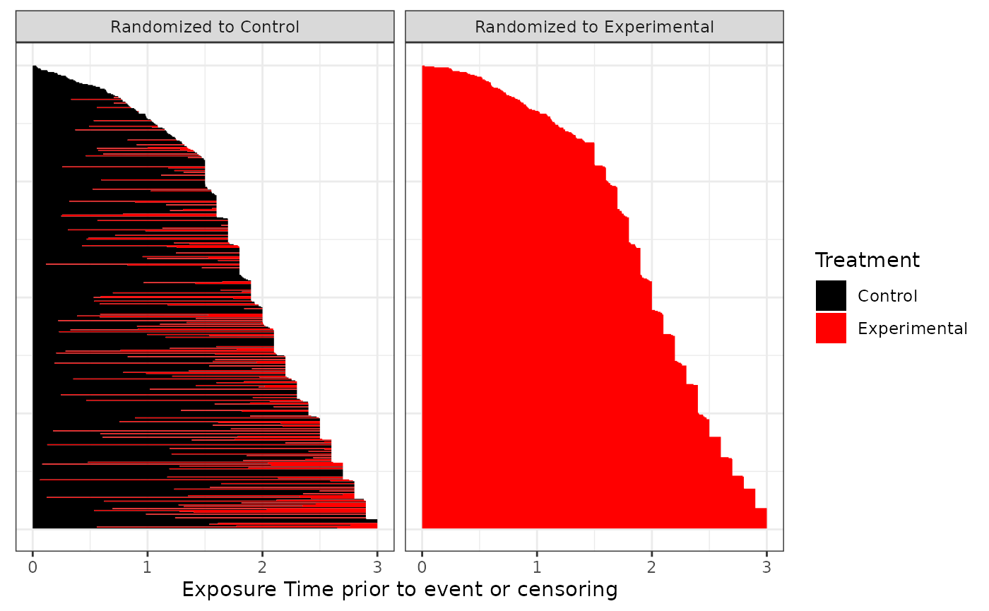

At risk plot and table

The second plot to consider shows the patient status over time. These are mutually exclusive states. I.e. the total percent of patients at risk is the sum of patients at risk on control and experimental.

ggatrisk(imm.fit)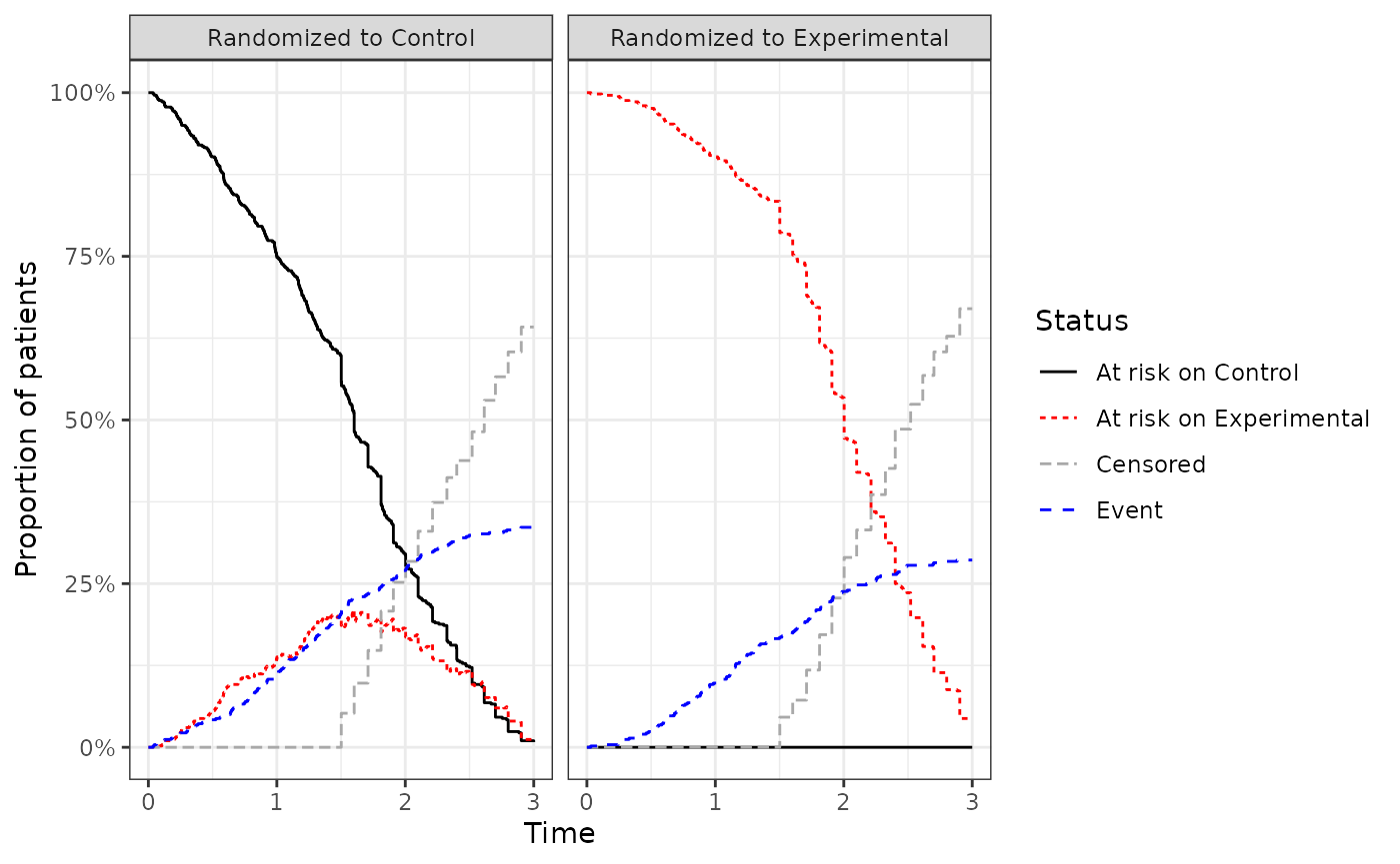

The plot data can be retrieved using the rpsftm.atrisk() function for tabulation.

rpsftm.atrisk(imm.fit, eval.times = c(0,1,2,3)) %>%
  dcast(Arm + Status ~ Time, value.var = "Count") %>%
  pander::pander()

Arm	Status	0	1	2	3
Randomized to Control	At risk on Control	500	375	147	4
Randomized to Control	At risk on Experimental	0	68	92	6
Randomized to Control	Censored	0	0	126	321
Randomized to Control	Event	0	57	135	169
Randomized to Experimental	At risk on Control	0	0	0	0
Randomized to Experimental	At risk on Experimental	500	451	267	22
Randomized to Experimental	Censored	0	0	114	335
Randomized to Experimental	Event	0	49	119	143

Discount Plot

This plot allows an assessment of the impact of switching. It shows hypothetical results for different levels of discount. A flat line indicates no impact of switching on results while a sloping line indicates that the switch does affect the results.

ggdiscount(imm.fit)
#> Warning: `data_frame()` was deprecated in tibble 1.1.0.
#> Please use `tibble()` instead.
#> This warning is displayed once every 8 hours.
#> Call `lifecycle::last_lifecycle_warnings()` to see where this warning was generated.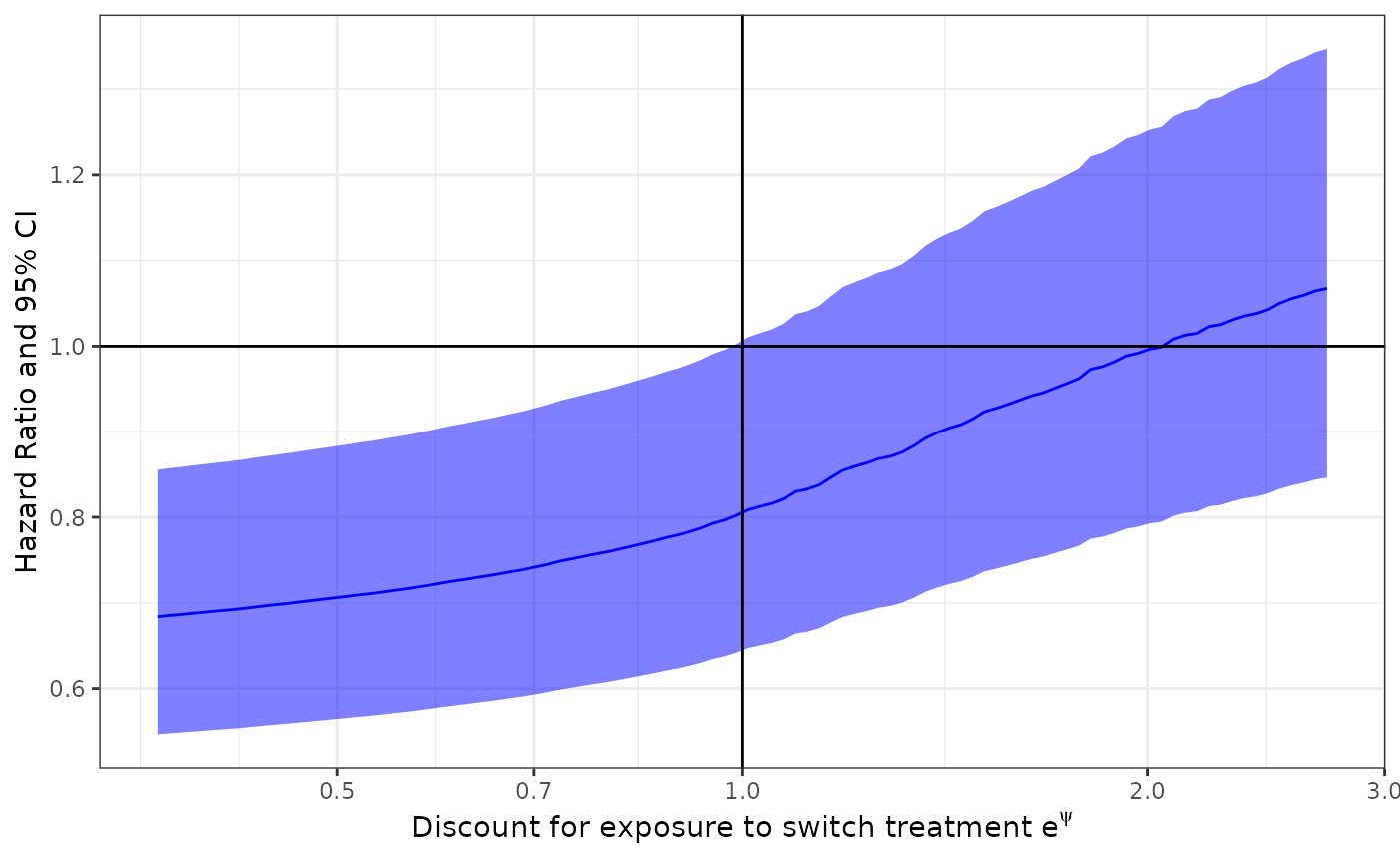

Diagnostic plots

The following plots are useful to assess if an rpsftm model has converged.

Psi plot

This shows the evaluated values of psi in the g-estimation. For convergence should be a single root. In this case it appears fine.

ggpsi(imm.fit)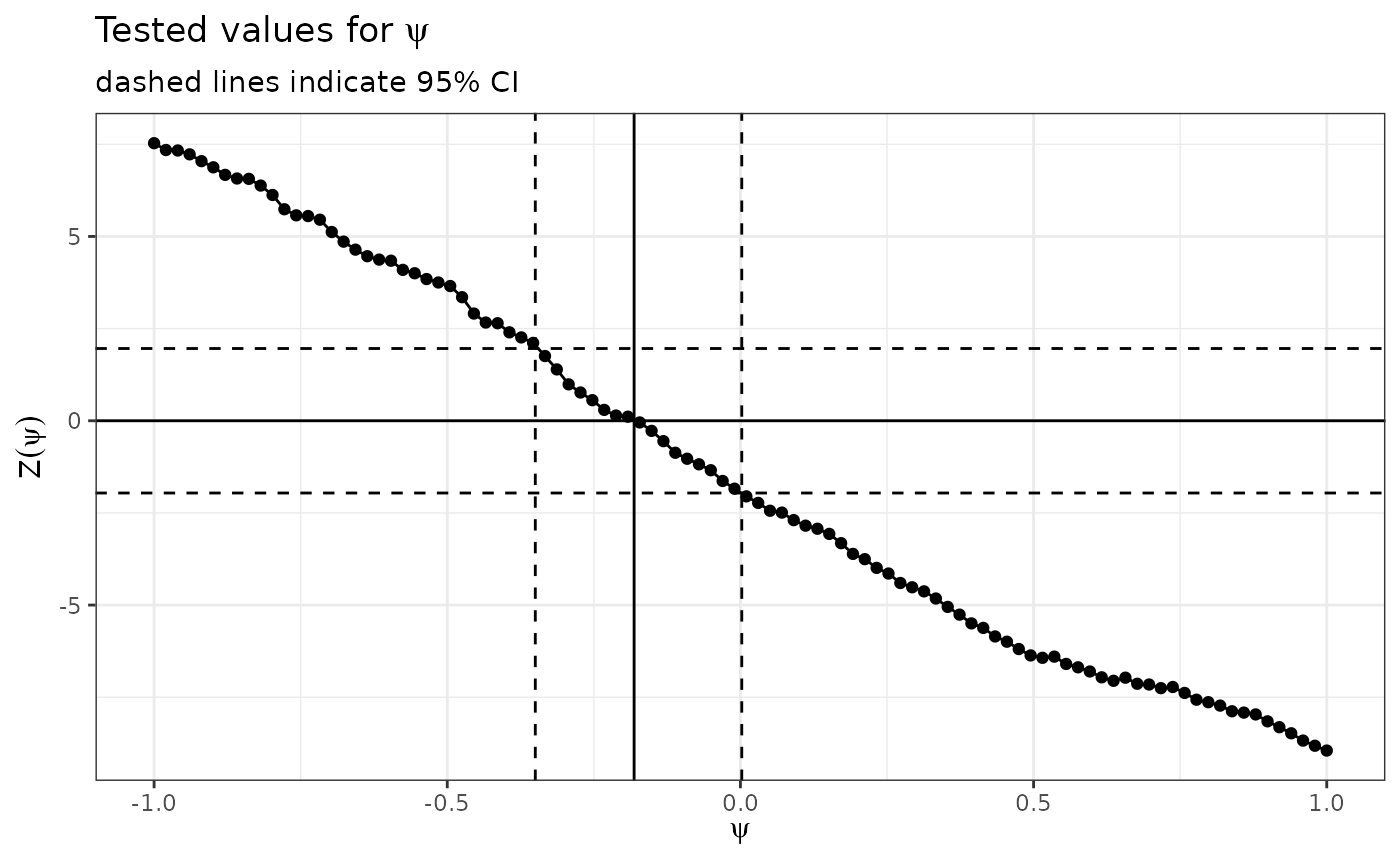

Latent survival plot

This shows the latent survival times for both arms. For convergence should be a overlapping per randomization. In this case it appears fine.

gglatent(imm.fit)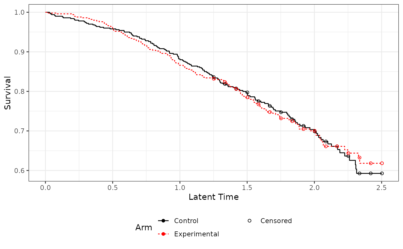

Result reporting

Assumming all diagnostics are fine and switching does impact the results can now look at the rpsftm results.

Survival plot

This shows the observed survival for both arms alongside the latent survial time for the control arm (as detected by rpsftm).

ggcfact(imm.fit)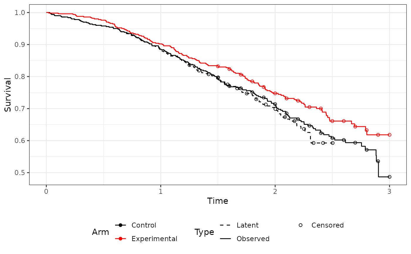

Cox model

This function fits a cox model comparing the observed experimental time to latent control time. Importantly it corrects the variance of the coefficient to account for the g-estimation procedure i.e. it inflates the variance based on the itt p-value.

rpsftm.coxph(imm.fit) %>%
  summary()
#> Call:
#> coxph(formula = rpsftm.formula(x), data = cfact.df)
#> 
#>   n= 1000, number of events= 285 
#> 
#>         coef exp(coef) se(coef)      z Pr(>|z|)  
#> .arm -0.2633    0.7685   0.1376 -1.914   0.0556 .
#> ---
#> Signif. codes:  0 '***' 0.001 '**' 0.01 '*' 0.05 '.' 0.1 ' ' 1
#> 
#>      exp(coef) exp(-coef) lower .95 upper .95
#> .arm    0.7685      1.301    0.5869     1.006
#> 
#> Concordance= 0.529  (se = 0.016 )
#> Likelihood ratio test= 4.72  on 1 df,   p=0.03
#> Wald test            = 4.72  on 1 df,   p=0.03
#> Score (logrank) test = 4.74  on 1 df,   p=0.03

Sensitivity of common treatment effect

This function refits an rpsft model with modified treatment effect in the control arm. This allows assessment of the sensitivity to the common treatment effect assumption.

# 50% efficacy for switchers
imm.fit.s1 <- rpsftm.refit(imm.fit, k = 0.5) 
imm.fit.s1 %>% rpsftm.coxph() %>% summary()
#> Call:
#> coxph(formula = rpsftm.formula(x), data = cfact.df)
#> 
#>   n= 1000, number of events= 300 
#> 
#>         coef exp(coef) se(coef)      z Pr(>|z|)  
#> .arm -0.2453    0.7825   0.1282 -1.914   0.0556 .
#> ---
#> Signif. codes:  0 '***' 0.001 '**' 0.01 '*' 0.05 '.' 0.1 ' ' 1
#> 
#>      exp(coef) exp(-coef) lower .95 upper .95
#> .arm    0.7825      1.278    0.6086     1.006
#> 
#> Concordance= 0.528  (se = 0.015 )
#> Likelihood ratio test= 4.44  on 1 df,   p=0.04
#> Wald test            = 4.43  on 1 df,   p=0.04
#> Score (logrank) test = 4.45  on 1 df,   p=0.03

# 80% efficacy for switchers
imm.fit.s2 <- rpsftm.refit(imm.fit, k = 0.8) 
imm.fit.s2 %>% rpsftm.coxph() %>% summary()
#> Call:
#> coxph(formula = rpsftm.formula(x), data = cfact.df)
#> 
#>   n= 1000, number of events= 292 
#> 
#>         coef exp(coef) se(coef)      z Pr(>|z|)  
#> .arm -0.2688    0.7643   0.1404 -1.914   0.0556 .
#> ---
#> Signif. codes:  0 '***' 0.001 '**' 0.01 '*' 0.05 '.' 0.1 ' ' 1
#> 
#>      exp(coef) exp(-coef) lower .95 upper .95
#> .arm    0.7643      1.308    0.5804     1.006
#> 
#> Concordance= 0.53  (se = 0.015 )
#> Likelihood ratio test= 5.1  on 1 df,   p=0.02
#> Wald test            = 5.1  on 1 df,   p=0.02
#> Score (logrank) test = 5.13  on 1 df,   p=0.02