Example for a Markov Model

Introduction

This document runs a discrete event simulation model in the context of a simple cohort Markov model with 4 states. Note that this same exercise could be done from a patient simulation approach rather than the cohort one.

Main options

library(descem)

library(dplyr)
#> 
#> Attaching package: 'dplyr'
#> The following objects are masked from 'package:stats':
#> 
#>     filter, lag
#> The following objects are masked from 'package:base':
#> 
#>     intersect, setdiff, setequal, union
library(flexsurv)
#> Loading required package: survival
library(ggplot2)
library(kableExtra)
#> 
#> Attaching package: 'kableExtra'
#> The following object is masked from 'package:dplyr':
#> 
#>     group_rows
library(purrr)
library(tidyr)

#Show all numbers, no scientific notation
options(scipen = 999)

Model Concept

The model is a simple Markov model with 4 states whose transition matrix can be found below. In order to run a pure Markov model within these functions, we will define each event as each cycle. We will generate an initial trace and at each event (cycle) we will update the trace by multiplying it by the transition matrix. Costs and QALYs can be computed in a similar fashion by multiplying the trace times the cost and the utility.

Load Data

The dummy data is generated below. The data structure should be as defined below, otherwise it will give problems.

#Utilities
util.data <- data.frame( name = c("util1" ,"util2" ,"util3" ,"util4"),
                         value = c(0.9,0.75,0.6,0),
                         se=rep(0.02,4),
                         stringsAsFactors = FALSE
)


#Costs
cost.data <- data.frame( name = c("cost1" ,"cost2" ,"cost3" ,"cost4","cost_int"),
                         value = c(1000,3000,6000,0,1000),
                         stringsAsFactors = FALSE
) %>%
  mutate(se= value/5)

General inputs with delayed execution

Initial inputs and flags that will be used in the model can be defined below. We can define inputs that are common to all patients (common_all_inputs) within a simulation, inputs that are unique to a patient independently of the treatment (e.g. natural death, defined in common_pt_inputs), and inputs that are unique to that patient and that treatment (unique_pt_inputs). Items can be included through the add_item function, and can be used in subsequent items. All these inputs are generated before the events and the reaction to events are executed. Furthermore, the program first executes common_all_inputs, then common_pt_inputs and then unique_pt_inputs. So one could use the items generated in common_all_inputs in unique_pt_inputs.

We also define here the specific utilities and costs that will be used in the model. It is strongly recommended to assign unnamed objects if they are going to be processed in the model. In this case, we’re only using util_v and cost_v as an intermediate input and these objects will not be processed (we just use them to make the code more readable), so it’s fine if we name them.

We define here our initial trace, the number of cycles to be simulated, the transition matrices and the initial cycle time (i.e. 0).

#Put objects here that do not change on any patient or intervention loop, for example a HR
common_all_inputs <- add_item(max_n_cycles = 30) %>%
  add_item( #utilities
    util_v = if(psa_bool){
      setNames(draw_gamma(util.data$value,util.data$se^2),util.data$name) #in this case I choose a gamma distribution
    } else{setNames(util.data$value,util.data$name)},
    util1 = util_v[["util1"]], 
    util2 = util_v[["util2"]],
    util3 = util_v[["util3"]],
    util4 = util_v[["util4"]]) %>%
  add_item( #costs
    cost_v = if(psa_bool){
      setNames(draw_gamma(cost.data$value,cost.data$se),cost.data$name) #in this case I choose a gamma distribution
    } else{setNames(cost.data$value,cost.data$name)},
    cost1    = cost_v[["cost1"]],
    cost2    = cost_v[["cost2"]],
    cost3    = cost_v[["cost3"]],
    cost4    = cost_v[["cost4"]],
    cost_int = cost_v[["cost_int"]])


#Put objects here that change as we loop through treatments for each patient (e.g. events can affect fl.tx, but events do not affect nat.os.s)
#common across trt but changes per pt could be implemented here (if (trt==)... )
unique_pt_inputs <- add_item(
                            trace = c(1,0,0,0),
                            transition = if( trt=="noint"){ 
                                            matrix(c(0.4,0.3,0.2,0.1,
                                            0.1,0.4,0.3,0.2,
                                            0.1,0.1,0.5,0.3,
                                            0,0,0,1),nrow=4,byrow=T)
                                         } else{
                                            matrix(c(0.5,0.3,0.1,0.1,
                                                     0.2,0.4,0.3,0.1,
                                                     0.1,0.2,0.5,0.2,
                                                     0,0,0,1),nrow=4,byrow=T)
                                              },
                            cycle_time = 0
)

Events

Add Initial Events

In our model, the events are start and cycle.

init_event_list <- 
  add_tte(trt="noint",evts=c("start","cycle"),input={ #intervention
    start <- 0
    
    cycle <- 1
    
  }) %>%
  add_tte(trt="int",evts=c("start","cycle"),input={ #intervention
    start <- 0
    
    cycle <- 1
   
    })

Add Reaction to Those Events

The explanation on how these part works can be seen in the early breast cancer tutorial.

In this Markov model case, in the event start we generate as many cycles as we need. At each cycle event we update the time of the cycle to keep track of it when we produce the output of the model and we update the trace. Finally, when all the events are over, we finish the simulation by setting curtime to infinity.


evt_react_list <-
  add_reactevt(name_evt = "start",
               input = {
                 for (i in 2:max_n_cycles) {
                   new_event(list("cycle" = curtime + i))
                 }
                 
               }) %>%
  add_reactevt(name_evt = "cycle",
               input = {
                 modify_item(list("cycle_time" = cycle_time + 1)) #Update cycle time
                 
                 modify_item(list( "trace" = trace %*% transition)) #Update trace
                 
                 if (max_n_cycles == cycle_time) {
                   modify_item(list("curtime" = Inf)) #Indicate end of simulation for patient
                 }
               })

Costs and Utilities

Costs and utilities are introduced below. However, it’s worth noting that the model is able to run without costs or utilities. One would just need to define the all the utility and costs related objects as NULL and the model would automatically assume they take value 0.

Utilities

Utilities are defined using pipes with the add_util function. In this case case, we are just multiplying the trace times the utilities at each state.



util_ongoing <- add_util(evt = c("start","cycle"),
                              trt = c("int", "noint"),
                              util = trace %*% c(util1,util2,util3,util4)
) #common utility across arms

Costs

Costs are defined using pipes with the add_cost function, in a similar fashion to the utilities. In this case we add the costs in a continuous fashion.


cost_ongoing <-
  add_cost(
    evt = c("start","cycle") ,
    trt = "noint",
    cost = trace %*% c(cost1,cost2,cost3,cost4)) %>%
  add_cost(
    evt = c("start","cycle") ,
    trt = "int",
    cost = trace %*% c(cost1+ cost_int,cost2+ cost_int,cost3+ cost_int,cost4) )

Model

Model Execution

The model can be run using the function RunSim below. We must define the number of patients to be simulated, the number of simulations, whether we want to run a PSA or not, the strategy list, the inputs, events and reactions defined above, the number of cores to be used (by default uses 1 core), the discount rate for costs and the discount rate for qalys. It is recommended not to use all the cores in the machine.

It is worth noting that the psa_bool argument does not run a PSA automatically, but is rather an additional input/flag of the model that we use as a reference to determine whether we want to use a deterministic or stochastic input. As such, it could also be defined in common_all_inputs as the first item to be defined, and the result would be the same. However, we recommend it to be defined in RunSim.

Note that the distribution chosen, the number of events and the interaction between events can have a substantial impact on the running time of the model. Since we are taking a cohort approach, we just need to indicate npats = 1.

#Logic is: per patient, per intervention, per event, react to that event.
results <- RunSim(  
  npats=1,                               # number of patients, recommended to set to 1000 if using PSA as it takes quite a while
  n_sim=1,                                  # if >1, then PSA, otherwise deterministic
  psa_bool = FALSE,
  trt_list = c("int", "noint"),             # intervention list
  common_all_inputs = common_all_inputs,    # inputs common that do not change within a simulation
  unique_pt_inputs = unique_pt_inputs,      # inputs that change within a simulation between interventions
  init_event_list = init_event_list,        # initial event list
  evt_react_list = evt_react_list,          # reaction of events
  util_ongoing_list = util_ongoing,
  cost_ongoing_list = cost_ongoing,
  ncores = 1,                               # number of cores to use, recommended not to use all
  drc = 0.035,                              # discount rate for costs
  drq = 0.035,                              # discount rate for QALYs
  input_out = c(                            # list of additional outputs (Flags, etc) that the user wants to export for each patient and event
    "trace",
    "cycle_time"
  )
)
#> [1] "Simulation number: 1"
#> Warning in RunSim(npats = 1, n_sim = 1, psa_bool = FALSE, trt_list = c("int", :
#> Item util_v is named. It is strongly advised to assign unnamed objects if they
#> are going to be processed in the model, as they can create errors depending on
#> how they are used within the model
#> Warning in RunSim(npats = 1, n_sim = 1, psa_bool = FALSE, trt_list = c("int", :
#> Item cost_v is named. It is strongly advised to assign unnamed objects if they
#> are going to be processed in the model, as they can create errors depending on
#> how they are used within the model
#> [1] "Time to run iteration 1: 0.23s"
#> [1] "Total time to run: 0.23s"

Post-processing of Model Outputs

Summary of Results

Once the model has been run, we can use the results and summarize them using the summary_results_det to print the results of the last simulation (if nsim=1, it’s the deterministic case), and summary_results_psa to show the PSA results (with the confidence intervals). We can also use the individual patient data generated by the simulation, which we collect here in the psa_ipd object. Note that the data for life years is wrong, as the model assumes we are running a patient simulation data and therefore it’s adding the 4 states, inflating the total life years. We can manually adjust this to get the correct life years.


summary_results_det(results$final_output) #will print the last simulation!
#>            int    noint
#> costs 24279.14 13956.96
#> lys      18.71    18.71
#> qalys     4.94     3.53
#> ICER        NA      Inf
#> ICUR        NA  7293.44

psa_ipd_simple <- bind_rows(map(results$output_psa, "merged_df")) %>% select(-trace) %>% distinct() 

psa_ipd <- bind_rows(map(results$output_psa, "merged_df")) 

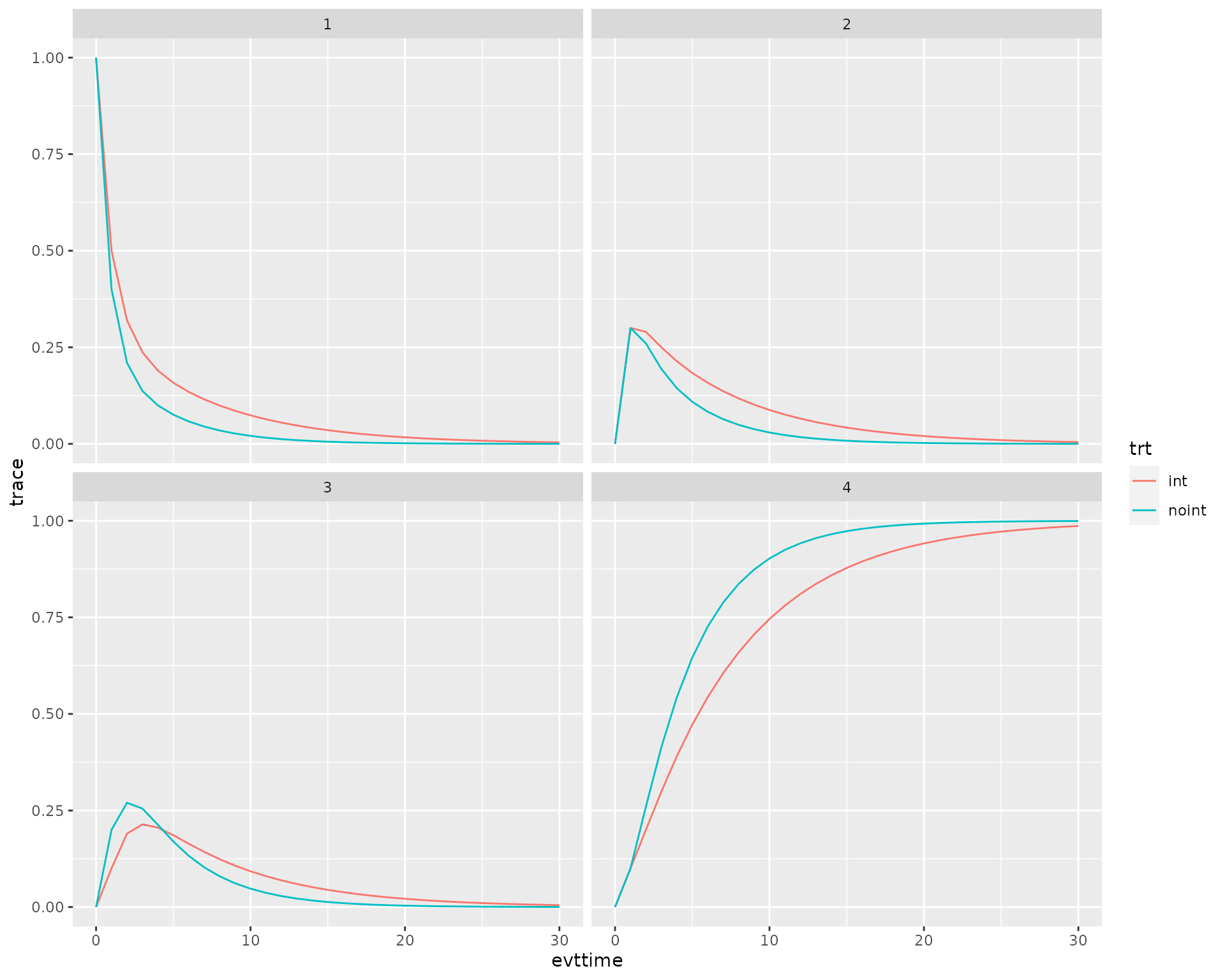
trace_t <- psa_ipd %>% mutate(state = rep(seq(1:4),62)) %>% select(trt,trace,state,evttime) 

trace_t[1:10,] %>%
  kable() %>%
  kable_styling(bootstrap_options = c("striped", "hover", "condensed", "responsive"))

trt	trace	state	evttime
int	1.00	1	0
int	0.00	2	0
int	0.00	3	0
int	0.00	4	0
int	0.50	1	1
int	0.30	2	1
int	0.10	3	1
int	0.10	4	1
int	0.32	1	2
int	0.29	2	2


life_years <-  psa_ipd %>%
  mutate(state = rep(seq(1:4),62)) %>% 
  group_by(trt) %>%
  filter(state!=4) %>% #erase death state for LY computation
  mutate(ly_final = ly*lag(trace,3L)) %>% #multiply by previous trace
summarise(ly_final = sum(ly_final,na.rm = TRUE)) #get final discounted life years

life_years %>%
  kable() %>%
  kable_styling(bootstrap_options = c("striped", "hover", "condensed", "responsive"))

trt	ly_final
int	6.329737
noint	4.584405


results$final_output[["lys.int"]] <- life_years$ly_final[life_years$trt=="int"]
results$final_output[["lys.noint"]] <- life_years$ly_final[life_years$trt=="noint"]

summary_results_det(results$final_output) #will print the last simulation!
#>            int    noint
#> costs 24279.14 13956.96
#> lys       6.33     4.58
#> qalys     4.94     3.53
#> ICER        NA  5914.16
#> ICUR        NA  7293.44

We can also check each of the cycles

evtname	evttime	cost	qaly	ly	pat_id	trt	cycle_time	total_costs	total_qalys	total_lys	simulation
start	0	0.000000	0.0000000	0.0000000	1	int	0	24279.14	4.943779	18.71206	1
cycle	1	1965.989690	0.8846954	0.9829948	1	int	1	24279.14	4.943779	18.71206	1
cycle	2	2754.285073	0.6980688	0.9497535	1	int	2	24279.14	4.943779	18.71206	1
cycle	3	2872.201325	0.5684756	0.9176362	1	int	3	24279.14	4.943779	18.71206	1
cycle	4	2634.990149	0.4691914	0.8866050	1	int	4	24279.14	4.943779	18.71206	1
cycle	5	2291.724094	0.3895537	0.8566232	1	int	5	24279.14	4.943779	18.71206	1
cycle	6	1947.762559	0.3242989	0.8276553	1	int	6	24279.14	4.943779	18.71206	1
cycle	7	1638.647105	0.2703019	0.7996669	1	int	7	24279.14	4.943779	18.71206	1
cycle	8	1372.316934	0.2254192	0.7726251	1	int	8	24279.14	4.943779	18.71206	1
cycle	9	1146.914659	0.1880358	0.7464976	1	int	9	24279.14	4.943779	18.71206	1
cycle	10	957.644750	0.1568698	0.7212538	1	int	10	24279.14	4.943779	18.71206	1
cycle	11	799.272995	0.1308761	0.6968635	1	int	11	24279.14	4.943779	18.71206	1
cycle	12	666.965087	0.1091921	0.6732981	1	int	12	24279.14	4.943779	18.71206	1
cycle	13	556.510746	0.0911018	0.6505296	1	int	13	24279.14	4.943779	18.71206	1
cycle	14	464.330280	0.0760089	0.6285310	1	int	14	24279.14	4.943779	18.71206	1
cycle	15	387.411713	0.0634166	0.6072763	1	int	15	24279.14	4.943779	18.71206	1
cycle	16	323.232479	0.0529105	0.5867404	1	int	16	24279.14	4.943779	18.71206	1
cycle	17	269.684293	0.0441450	0.5668989	1	int	17	24279.14	4.943779	18.71206	1
cycle	18	225.006775	0.0368316	0.5477284	1	int	18	24279.14	4.943779	18.71206	1
cycle	19	187.730662	0.0307298	0.5292062	1	int	19	24279.14	4.943779	18.71206	1
cycle	20	156.629904	0.0256389	0.5113104	1	int	20	24279.14	4.943779	18.71206	1
cycle	21	130.681491	0.0213914	0.4940197	1	int	21	24279.14	4.943779	18.71206	1
cycle	22	109.031868	0.0178475	0.4773137	1	int	22	24279.14	4.943779	18.71206	1
cycle	23	90.968872	0.0148908	0.4611727	1	int	23	24279.14	4.943779	18.71206	1
cycle	24	75.898320	0.0124239	0.4455774	1	int	24	24279.14	4.943779	18.71206	1
cycle	25	63.324462	0.0103656	0.4305096	1	int	25	24279.14	4.943779	18.71206	1
cycle	26	52.833680	0.0086484	0.4159513	1	int	26	24279.14	4.943779	18.71206	1
cycle	27	44.080875	0.0072156	0.4018853	1	int	27	24279.14	4.943779	18.71206	1
cycle	28	36.778122	0.0060202	0.3882950	1	int	28	24279.14	4.943779	18.71206	1
cycle	29	30.685196	0.0050229	0.3751642	1	int	29	24279.14	4.943779	18.71206	1
cycle	30	25.601667	0.0041908	0.3624775	1	int	30	24279.14	4.943779	18.71206	1
start	0	0.000000	0.0000000	0.0000000	1	noint	0	13956.96	3.528511	18.71206	1
cycle	1	982.994845	0.8846954	0.9829948	1	noint	1	13956.96	3.528511	18.71206	1
cycle	2	2374.383683	0.6695762	0.9497535	1	noint	2	13956.96	3.528511	18.71206	1
cycle	3	2395.030498	0.5010294	0.9176362	1	noint	3	13956.96	3.528511	18.71206	1
cycle	4	1993.974713	0.3739700	0.8866050	1	noint	4	13956.96	3.528511	18.71206	1
cycle	5	1551.258984	0.2790364	0.8566232	1	noint	5	13956.96	3.528511	18.71206	1
cycle	6	1175.940902	0.2082166	0.8276553	1	noint	6	13956.96	3.528511	18.71206	1
cycle	7	882.644380	0.1553847	0.7996669	1	noint	7	13956.96	3.528511	18.71206	1
cycle	8	660.066030	0.1159643	0.7726251	1	noint	8	13956.96	3.528511	18.71206	1
cycle	9	492.963971	0.0865468	0.7464976	1	noint	9	13956.96	3.528511	18.71206	1
cycle	10	367.997323	0.0645925	0.7212538	1	noint	10	13956.96	3.528511	18.71206	1
cycle	11	274.668169	0.0482076	0.6968635	1	noint	11	13956.96	3.528511	18.71206	1
cycle	12	204.998719	0.0359790	0.6732981	1	noint	12	13956.96	3.528511	18.71206	1
cycle	13	152.998690	0.0268524	0.6505296	1	noint	13	13956.96	3.528511	18.71206	1
cycle	14	114.188546	0.0200409	0.6285310	1	noint	14	13956.96	3.528511	18.71206	1
cycle	15	85.223026	0.0149573	0.6072763	1	noint	15	13956.96	3.528511	18.71206	1
cycle	16	63.605003	0.0111631	0.5867404	1	noint	16	13956.96	3.528511	18.71206	1
cycle	17	47.470696	0.0083315	0.5668989	1	noint	17	13956.96	3.528511	18.71206	1
cycle	18	35.429084	0.0062181	0.5477284	1	noint	18	13956.96	3.528511	18.71206	1
cycle	19	26.441998	0.0046408	0.5292062	1	noint	19	13956.96	3.528511	18.71206	1
cycle	20	19.734613	0.0034636	0.5113104	1	noint	20	13956.96	3.528511	18.71206	1
cycle	21	14.728650	0.0025850	0.4940197	1	noint	21	13956.96	3.528511	18.71206	1
cycle	22	10.992521	0.0019293	0.4773137	1	noint	22	13956.96	3.528511	18.71206	1
cycle	23	8.204113	0.0014399	0.4611727	1	noint	23	13956.96	3.528511	18.71206	1
cycle	24	6.123024	0.0010746	0.4455774	1	noint	24	13956.96	3.528511	18.71206	1
cycle	25	4.569833	0.0008020	0.4305096	1	noint	25	13956.96	3.528511	18.71206	1
cycle	26	3.410630	0.0005986	0.4159513	1	noint	26	13956.96	3.528511	18.71206	1
cycle	27	2.545476	0.0004467	0.4018853	1	noint	27	13956.96	3.528511	18.71206	1
cycle	28	1.899780	0.0003334	0.3882950	1	noint	28	13956.96	3.528511	18.71206	1
cycle	29	1.417874	0.0002488	0.3751642	1	noint	29	13956.96	3.528511	18.71206	1
cycle	30	1.058210	0.0001857	0.3624775	1	noint	30	13956.96	3.528511	18.71206	1

Plots

We now use the data to plot the traces.


ggplot(trace_t,aes(x=evttime,y = trace,col=trt)) + geom_line() + facet_wrap(~state)

Javier Sanchez Alvarez and Valerie Aponte Ribero

July 26, 2022