Structural and Parametric Uncertainty
Javier Sanchez Alvarez and Valerie Aponte Ribero
July 26, 2022
example_uncertainty.RmdIntroduction
This document runs a discrete event simulation model in the context of early breast cancer to show how uncertainty behaves in a simulation setting and how it complements with a standard PSA. As the model is extremely similar to the example in early breast cancer, the user can check the original model for details on functions, parameters etc.
Main options
library(descem)

library(dplyr)
#>
#> Attaching package: 'dplyr'
#> The following objects are masked from 'package:stats':
#>
#>     filter, lag
#> The following objects are masked from 'package:base':
#>
#>     intersect, setdiff, setequal, union
library(purrr)
library(tidyr)
library(flexsurv)
#> Loading required package: survival
library(ggplot2)
library(kableExtra)
#>
#> Attaching package: 'kableExtra'
#> The following object is masked from 'package:dplyr':
#>
#> group_rowsGeneral inputs with delayed execution
Initial inputs and flags that will be used in the model can be defined below. This is exactly the same as in the original model, the only difference is that now we are adding an extra chunk which reflects the uncertainty of parameters to draw distributions. Furthermore, utilities and costs also have a distribution.
#Each patient is identified through "i"
#Items used in the model should be unnamed numeric/vectors! otherwise if they are processed by model it can lead to strangely named outcomes
#In this case, util_v is a named vector, but it's not processed by the model. We extract unnamed numerics from it.

#Put objects here that do not change on any patient or intervention loop
common_all_inputs <- add_item( #utilities
    util_v = if(psa_bool){
                     setNames(MASS::mvrnorm(1,util.data$value,diag(util.data$se^2)),util.data$name) #in this case I choose a multivariate normal with no correlation
             } else{setNames(util.data$value,util.data$name)},
    util.idfs.ontx = util_v[["util.idfs.ontx"]],
    util.idfs.offtx  = util_v[["util.idfs.offtx"]],
    util.remission = util_v[["util.remission"]],
    util.recurrence = util_v[["util.recurrence"]],
    util.mbc.progression.mbc = util_v[["util.mbc.progression.mbc"]],
    util.mbc.pps = util_v[["util.mbc.pps"]]
    ) %>%
  add_item( #costs
    cost_v = if(psa_bool){
                     setNames(draw_gamma(cost.data$value,cost.data$se),cost.data$name) #in this case I choose a gamma distribution
             } else{setNames(cost.data$value,cost.data$name)},
    cost.idfs.tx  = cost_v[["cost.idfs.tx"]],
    cost.recurrence  = cost_v[["cost.recurrence"]],
    cost.mbc.tx  = cost_v[["cost.mbc.tx"]],
    cost.tx.beva  = cost_v[["cost.tx.beva"]],
    cost.idfs.txnoint = cost_v[["cost.idfs.txnoint"]],
    cost.idfs = cost_v[["cost.idfs"]],
    cost.mbc.progression.mbc = cost_v[["cost.mbc.progression.mbc"]],
    cost.mbc.pps = cost_v[["cost.mbc.pps"]],
    cost.2ndline = cost_v[["cost.2ndline"]],
    cost.ae = cost_v[["cost.ae"]]
    ) %>%
  add_item( #parameter uncertainty
    coef11_psa = ifelse(psa_bool,rnorm(1,2,0.1),2),
    coef12_psa = ifelse(psa_bool,rnorm(1,3,0.1),3),
    coef13_psa = ifelse(psa_bool,rnorm(1,0.8,0.05),0.8),
    coef14_psa = ifelse(psa_bool,rnorm(1,0.5,0.05),0.5),
    coef15_psa = ifelse(psa_bool,rnorm(1,2.3,0.1),2.3),
    coef16_psa = ifelse(psa_bool,log(rnorm(1,0.08,0.005)),log(0.08)),
    coef2_psa = ifelse(psa_bool,log(rnorm(1,0.2,0.01)),log(0.2)),
    hr_psa = ifelse(psa_bool,exp(rnorm(1,log(1.2),0.05)),1.2)
    )

#Put objects here that do not change as we loop through interventions for a patient
common_pt_inputs <- add_item(sex_pt = ifelse(rbernoulli(1,p=0.01),"male","female"),
                             nat.os.s = draw_resgompertz(1,
                                                     shape=if(sex_pt=="male"){0.102}else{0.115},
                                                     rate=if(sex_pt=="male"){0.000016}else{0.0000041},
                                                     lower_bound = 50) ) #in years, for a patient who is 50yo

#Put objects here that change as we loop through treatments for each patient (e.g. events can affect fl.tx, but events do not affect nat.os.s)
#common across trt but changes per pt could be implemented here (if (trt==)... )
unique_pt_inputs <- add_item(
  fl.idfs.ontx             = 1,
  fl.idfs                  = 1,
  fl.mbcs.ontx             = 1,
  fl.mbcs.progression.mbc  = 1,
  fl.tx.beva               = 1,
  fl.mbcs                  = 0,
  fl.mbcs_2ndline          = 0,
  fl.recurrence            = 0,
  fl.remission             = rbernoulli(1,0.8) #80% probability of going into remission
)
Events
Add Initial Events
Events are generated as before, the only difference being that the parameters are not a simple number but the objects created as part of common_all_inputs.
init_event_list <-
  add_tte(trt="int",
               evts = c("start","ttot", "ttot.beva","progression.mbc", "os","idfs","ttot.early","remission","recurrence","start.early.mbc"),
               other_inp = c("os.early","os.mbc"),
               input={ #intervention
    start <- 0

    #Early

    idfs <- draw_tte(1,'lnorm',coef1=coef11_psa, coef2=coef2_psa)
    ttot.early <- min(draw_tte(1,'lnorm',coef1=coef11_psa, coef2=coef2_psa),idfs)
    ttot.beva <- draw_tte(1,'lnorm',coef1=coef11_psa, coef2=coef2_psa)

    os.early <- draw_tte(1,'lnorm',coef1=coef12_psa, coef2=coef2_psa)

    #if patient has remission, check when will recurrence happen
    if (fl.remission) {
      recurrence <- idfs + draw_tte(1,'lnorm',coef1=coef11_psa, coef2=coef2_psa)
      remission <- idfs

      #if recurrence happens before death
      if (min(os.early,nat.os.s)>recurrence) {

        #Late metastatic (after finishing idfs and recurrence)

        os.mbc <- draw_tte(1,'lnorm',coef1=coef13_psa, coef2=coef2_psa) + idfs  +  recurrence

        progression.mbc <- draw_tte(1,'lnorm',coef1=coef14_psa, coef2=coef2_psa) + idfs +  recurrence

        ttot <- draw_tte(1,'lnorm',coef1=coef14_psa, coef2=coef2_psa) + idfs +  recurrence


      }

    } else{ #If early metastatic
      start.early.mbc <- draw_tte(1,'lnorm',coef1=coef15_psa, coef2=coef2_psa)

      idfs <- ifelse(start.early.mbc<idfs,start.early.mbc,idfs)
      ttot.early <- min(ifelse(start.early.mbc<idfs,start.early.mbc,idfs),ttot.early)

      os.mbc <- draw_tte(1,'lnorm',coef1=coef13_psa, coef2=coef2_psa) + start.early.mbc

      progression.mbc <- draw_tte(1,'lnorm',coef1=coef14_psa, coef2=coef2_psa) + start.early.mbc

      ttot <- draw_tte(1,'lnorm',coef1=coef14_psa, coef2=coef2_psa) + start.early.mbc

    }

    os <- min(os.mbc,os.early,nat.os.s)


  }) %>%  add_tte(trt="noint",
                       evts = c("start","ttot", "ttot.beva","progression.mbc", "os","idfs","ttot.early","remission","recurrence","start.early.mbc"),
                       other_inp = c("os.early","os.mbc"),
                       input={  #reference strategy
    start <- 0

    #Early

    idfs <- draw_tte(1,'lnorm',coef1=coef11_psa, coef2=coef2_psa,hr=hr_psa)
    ttot.early <- min(draw_tte(1,'lnorm',coef1=coef11_psa, coef2=coef2_psa,hr=hr_psa),idfs)

    os.early <- draw_tte(1,'lnorm',coef1=coef12_psa, coef2=coef2_psa,hr=hr_psa)

    #if patient has remission, check when will recurrence happen
    if (fl.remission) {
      recurrence <- idfs +draw_tte(1,'lnorm',coef1=coef11_psa, coef2=coef2_psa)
      remission <- idfs

      #if recurrence happens before death
      if (min(os.early,nat.os.s)>recurrence) {

        #Late metastatic (after finishing idfs and recurrence)

        os.mbc <- draw_tte(1,'lnorm',coef1=coef13_psa, coef2=coef2_psa) + idfs  +  recurrence

        progression.mbc <- draw_tte(1,'lnorm',coef1=coef14_psa, coef2=coef2_psa) + idfs +  recurrence

        ttot <- draw_tte(1,'lnorm',coef1=coef14_psa, coef2=coef2_psa) + idfs +  recurrence

      }

    } else{ #If early metastatic
      start.early.mbc <- draw_tte(1,'lnorm',coef1=coef15_psa, coef2=coef2_psa)

      idfs <- ifelse(start.early.mbc<idfs,start.early.mbc,idfs)
      ttot.early <- min(ifelse(start.early.mbc<idfs,start.early.mbc,idfs),ttot.early)

      os.mbc <- draw_tte(1,'lnorm',coef1=coef13_psa, coef2=coef2_psa) + start.early.mbc

      progression.mbc <- draw_tte(1,'lnorm',coef1=coef14_psa, coef2=coef2_psa) + start.early.mbc

      ttot <- draw_tte(1,'lnorm',coef1=coef14_psa, coef2=coef2_psa) + start.early.mbc


    }
    os <- min(os.mbc,os.early,nat.os.s)

  })
Add Reaction to Those Events
The reactions are set in the same fashion as in the original model. A small modification has been made in generating the event 2ndline_mbc, which now also uses a random parameter if the PSA option is active.
evt_react_list <-
  add_reactevt(name_evt = "start",
               input = {}) %>%
  add_reactevt(name_evt = "ttot",
               input = {
                 modify_item(list("fl.mbcs.ontx"= 0)) #Flag that patient is now off-treatment

               }) %>%
  add_reactevt(name_evt = "ttot.beva",
               input = {
                 modify_item(list("fl.tx.beva"= 0)) #Flag that patient is now off-treatment

               }) %>%
  add_reactevt(name_evt = "progression.mbc",
               input = {
                 modify_item(list("fl.mbcs.progression.mbc"=0,"fl.mbcs_2ndline"=1)) #Flag that patient is progressed and going in 2nd line

                 new_event(list("2ndline_mbc" = curtime + draw_tte(1,'exp', coef16_psa)/12))

               }) %>%
  add_reactevt(name_evt = "idfs",
               input = {
                 modify_item(list("fl.idfs"= 0))

               }) %>%
  add_reactevt(name_evt = "ttot.early",
               input = {
                 modify_item(list("fl.idfs.ontx"=0,"fl.tx.beva"=0)) #Flag that patient is now off-treatment

                 n_ae <- rpois(1,lambda=0.25*(curtime -prevtime)) #1 AE every 4 years

                 if (n_ae>0) {
                   new_event(rep(list("ae" = curtime + 0.0001),n_ae))
                 }
               }) %>%
  add_reactevt(name_evt = "remission",
               input = {
                 modify_item(list("fl.remission"= 1))

               }) %>%
  add_reactevt(name_evt = "recurrence",
               input = {
                 modify_item(list("fl.recurrence"=1,"fl.remission"=0,"fl.mbcs"=1,"fl.mbcs.progression.mbc"=1)) #ad-hoc for plot

               }) %>%
  add_reactevt(name_evt = "start.early.mbc",
               input = {
                 modify_item(list("fl.mbcs"=1,"fl.mbcs.progression.mbc"=1))

               }) %>%
  add_reactevt(name_evt = "2ndline_mbc",
               input = {
                 modify_item(list("fl.mbcs_2ndline"= 0))

                 n_ae <- rpois(1,lambda=0.25*(curtime -prevtime)) #1 AE every 4 years

                 if (n_ae>0) {
                   new_event(rep(list("ae" = curtime + 0.0001),n_ae))
                 }
               }) %>%
  add_reactevt(name_evt = "ae",
               input = {
                 modify_event(list("os" =max(cur_evtlist[["os"]] - 0.125,curtime +0.0001) ))#each AE brings forward death by 1.5 months
               }) %>%
  add_reactevt(name_evt = "os",
               input = {
                 modify_item(list("fl.tx.beva"=0,"fl.mbcs.ontx"=0,"fl.idfs"=0,"fl.mbcs"=0,"curtime"=Inf))
               })
Costs and Utilities
Costs and utilities are introduced below.
util_ongoing <- add_util(evt = c("start","ttot","ttot.beva","progression.mbc","os","idfs","ttot.early","remission","recurrence","start.early.mbc","2ndline_mbc","ae"),
                              trt = c("int", "noint"),
                              util = if (fl.idfs==1) {
                                util.idfs.ontx * fl.idfs.ontx + (1-fl.idfs.ontx) * (1-fl.idfs.ontx)
                              } else if (fl.idfs==0 & fl.mbcs==0) {
                                util.remission * fl.remission + fl.recurrence*util.recurrence
                              } else if (fl.mbcs==1) {
                                util.mbc.progression.mbc * fl.mbcs.progression.mbc + (1-fl.mbcs.progression.mbc)*util.mbc.pps
                              }
)

cost_ongoing <-
  add_cost(
    evt = c("start","idfs","ttot.early") ,
    trt = "noint",
    cost = cost.idfs.txnoint* fl.idfs.ontx  + cost.idfs) %>%
  add_cost(
    evt = c("start","idfs","ttot.early") ,
    trt = "int",
    cost = (cost.idfs.tx) * fl.idfs.ontx + cost.tx.beva * fl.tx.beva + cost.idfs) %>%
  add_cost(
    evt = c("remission","recurrence","start.early.mbc"),
    trt = c("noint","int"),
    cost = cost.recurrence * fl.recurrence) %>%
  add_cost(
    evt = c("ttot","ttot.beva","progression.mbc","os","2ndline_mbc"),
    trt = c("noint","int"),
    cost = cost.mbc.tx  * fl.mbcs.ontx + cost.mbc.progression.mbc * fl.mbcs.progression.mbc + cost.mbc.pps * (1-fl.mbcs.progression.mbc) + cost.2ndline*fl.mbcs_2ndline  )


cost_instant <-  add_cost(
  evt = c("ae"),
  trt = c("noint","int"),
  cost = cost.ae)
Model
The model can now be executed as normal. Given that this modeling exercise relies on sampling from distributions and simulating a finite number of patients, there is some randomness involved that can affect the results, even under the assumption that the parameters are fixed. However, running more patients also means the simulation is slower, so there is a trade-off between accuracy and speed. An important question here is to understand how much of the uncertainty we observe when running a PSA comes from the parametric uncertainty and how much comes from the fact that we are simulating a finite sample.
Structural Uncertainty
One way to test this is to run a few simulations for an increasing number of patients simulated. For example, below we run 50 deterministic simulations for 100, 1,000, 5,000 and 10,000 patients, to show how the model outcome can change depending on the random seed used. Note that this exercise can be very time consuming. It’s important to note that the optimal number of patients simulated will depend on the dispersion of the distributions, the patient pathway, the number of possible outcomes and the difference among these. For example, an event with low probability but high impact and variability implies a higher number of patients simulated in order to obtain stable outcomes.
To do this test, we set psa_bool = FALSE and (optional) we set ipd = FALSE. This last option means that we are not exporting IPD data from all these simulations, but rather the aggregate outcomes (and the last simulation, which is included by default). This is important when simulating a large number of patients with a lot of simulations, which can generate very large objects (>1 GB). This option can also be especially relevant when running a PSA, which would require psa_bool = TRUE and a high number of simulations.
sample_sizes <- c(100,1000,2000,5000)

sim_size_df <- NULL
for (sample_size in sample_sizes) {
  results <- suppressWarnings( #run without warnings
      RunSim(
    npats=sample_size,                        # number of patients to be simulated
    n_sim=50,                                # number of simulations to run
    psa_bool = FALSE,                         # use PSA or not. If n_sim > 1 and psa_bool = FALSE, then difference in outcomes is due to sampling (number of pats simulated)
    trt_list = c("int", "noint"),             # intervention list
    common_all_inputs = common_all_inputs,    # inputs common that do not change within a simulation
    common_pt_inputs = common_pt_inputs,      # inputs that change within a simulation but are not affected by the intervention
    unique_pt_inputs = unique_pt_inputs,      # inputs that change within a simulation between interventions
    init_event_list = init_event_list,        # initial event list
    evt_react_list = evt_react_list,          # reaction of events
    util_ongoing_list = util_ongoing,
    cost_ongoing_list = cost_ongoing,
    cost_instant_list = cost_instant,
    ncores = min(parallel::detectCores() -1,30), # number of cores to use, recommended not to use all
    drc = 0.035,                              # discount rate for costs
    drq = 0.035,                              # discount rate for qalys
    ipd=FALSE                                 # Return IPD data through merged_df? Set to FALSE as it's not of interest here and it makes code slower
  ))

  #We're extracting the overall ICER/ICUR and also costs/qalys/lys for the "noint" intervention
  loop_df <- rbind(extract_psa_result(results$output_psa,"costs","noint"),
                   extract_psa_result(results$output_psa,"lys","noint"),
                   extract_psa_result(results$output_psa,"qalys","noint"),
                   extract_psa_result(results$output_psa,"costs","int"),
                   extract_psa_result(results$output_psa,"lys","int"),
                   extract_psa_result(results$output_psa,"qalys","int"))

    loop_df <- rbind(loop_df, loop_df %>%
                     spread(trt,value) %>%
                     mutate(dif = int - noint) %>%
                     group_by(simulation) %>%
                     transmute(value = dif[element=="costs"]/dif[element=="qalys"],element = "ICUR", trt="noint") %>%
                     relocate(element, trt) %>%
                     ungroup() %>%
                     distinct())


  loop_df$sample_size = sample_size
  sim_size_df <- rbind(sim_size_df,loop_df)

}
We can then plot the results (in this case, the costs, lys and qalys are for the “noint” intervention) 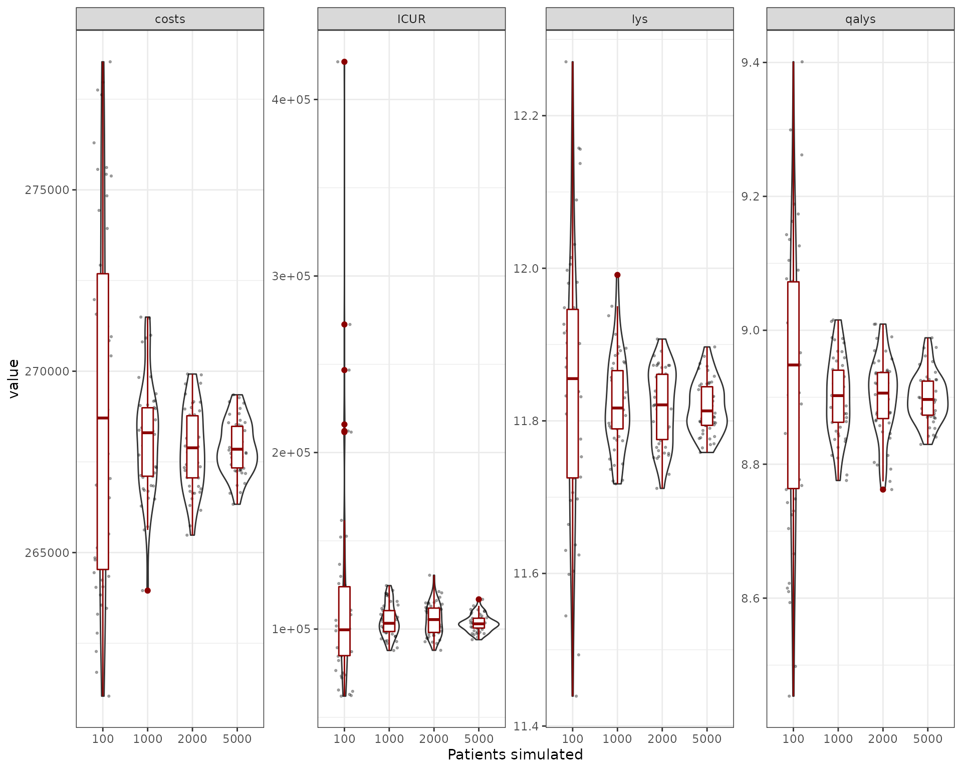
We can also try to understand what is the relative size of the uncertainty provided by the sampling. We compute the coefficient of variation for the outcomes exported (costs, qalys, lys, ICER and ICUR). The first thing to be noticed is that the ICER and ICUR CV is much higher than for costs/lys/qalys. This is because of the incremental nature of ICER/ICUR, which means it’s more sensitive to small variations of these outputs. So while the costs/qalys/lys are quite precise with a reduced number of simulations (~1,000), in order to have a precise ICER/ICUR we need to go higher (~5,000/10,000). However, one can see that the mean is quite stable at ~5,000 patients.
| element | sample_size | mean | sd | CV (%) |
|---|---|---|---|---|
| costs | 100 | 269158.30 | 4992.73 | 1.85 |
| costs | 1000 | 268150.76 | 1531.52 | 0.57 |
| costs | 2000 | 267860.84 | 1108.74 | 0.41 |
| costs | 5000 | 267906.69 | 729.69 | 0.27 |
| ICUR | 100 | 117871.37 | 64331.40 | 54.58 |
| ICUR | 1000 | 104710.13 | 9119.97 | 8.71 |
| ICUR | 2000 | 105163.13 | 8985.53 | 8.54 |
| ICUR | 5000 | 103316.11 | 4782.38 | 4.63 |
| lys | 100 | 11.84 | 0.18 | 1.49 |
| lys | 1000 | 11.82 | 0.06 | 0.52 |
| lys | 2000 | 11.82 | 0.05 | 0.41 |
| lys | 5000 | 11.82 | 0.03 | 0.29 |
| qalys | 100 | 8.92 | 0.21 | 2.35 |
| qalys | 1000 | 8.90 | 0.06 | 0.66 |
| qalys | 2000 | 8.90 | 0.06 | 0.65 |
| qalys | 5000 | 8.90 | 0.04 | 0.41 |
We can plot the CV to see this more clearly: 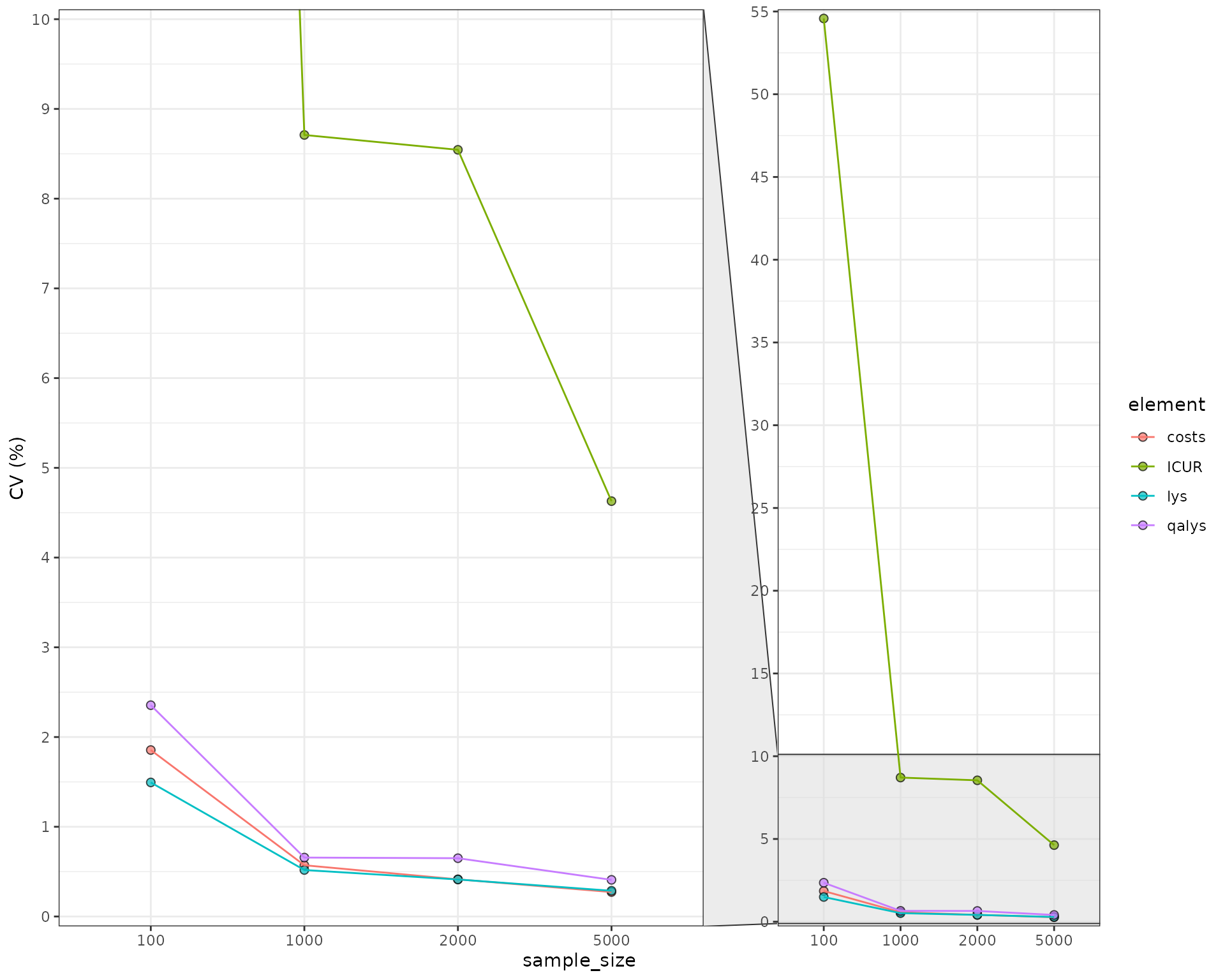
Parameter Uncertainty
Structural uncertainty is not the only type of uncertainty that the model can have. Parameters can also be changed across simulations by using the psa_bool = TRUE option. Let’s see what happens when we compare the true PSA to the structural uncertainty with 1,000 patients.
sample_sizes <- 1000

sim_size_psa_df <- NULL
for (sample_size in sample_sizes) {
  results <- suppressWarnings(RunSim(
    npats=sample_size,                        # number of patients to be simulated
    n_sim=50,                                # number of simulations to run
    psa_bool = TRUE,                         # use PSA or not. If n_sim > 1 and psa_bool = FALSE, then difference in outcomes is due to sampling (number of pats simulated)
    trt_list = c("int", "noint"),             # intervention list
    common_all_inputs = common_all_inputs,    # inputs common that do not change within a simulation
    common_pt_inputs = common_pt_inputs,      # inputs that change within a simulation but are not affected by the intervention
    unique_pt_inputs = unique_pt_inputs,      # inputs that change within a simulation between interventions
    init_event_list = init_event_list,        # initial event list
    evt_react_list = evt_react_list,          # reaction of events
    util_ongoing_list = util_ongoing,
    cost_ongoing_list = cost_ongoing,
    cost_instant_list = cost_instant,
    ncores = min(parallel::detectCores() -1,30),      # number of cores to use, recommended not to use all
    drc = 0.035,                              # discount rate for costs
    drq = 0.035,                              # discount rate for qalys
    ipd=FALSE                                 # Return IPD data through merged_df? Set to FALSE as it's not of interest here and it makes code slower
  ))

  #We're extracting the overall ICER/ICUR and also costs/qalys/lys for the "noint" intervention
  loop_psa_df <- rbind(extract_psa_result(results$output_psa,"costs","noint"),
                   extract_psa_result(results$output_psa,"lys","noint"),
                   extract_psa_result(results$output_psa,"qalys","noint"),
                   extract_psa_result(results$output_psa,"costs","int"),
                   extract_psa_result(results$output_psa,"lys","int"),
                   extract_psa_result(results$output_psa,"qalys","int"))

    loop_psa_df <- rbind(loop_psa_df, loop_psa_df %>%
                     spread(trt,value) %>%
                     mutate(dif = int - noint) %>%
                     group_by(simulation) %>%
                     transmute(value = dif[element=="costs"]/dif[element=="qalys"],element = "ICUR", trt="noint") %>%
                     relocate(element, trt) %>%
                     ungroup() %>%
                     distinct())

  loop_psa_df$sample_size = sample_size
  sim_size_psa_df <- rbind(sim_size_psa_df,loop_psa_df)

}
Now the uncertainty is much bigger when compared to the same case with 1,000 iterations and no parameter uncertainty.
| element | sample_size | uncertainty | mean | sd | CV (%) |
|---|---|---|---|---|---|
| costs | 1000 | structural | 268150.76 | 1531.52 | 0.57 |
| costs | 1000 | structural + parameter | 261114.34 | 37150.02 | 14.23 |
| ICUR | 1000 | structural | 104710.13 | 9119.97 | 8.71 |
| ICUR | 1000 | structural + parameter | 111738.55 | 51806.93 | 46.36 |
| lys | 1000 | structural | 11.82 | 0.06 | 0.52 |
| lys | 1000 | structural + parameter | 11.79 | 0.47 | 4.00 |
| qalys | 1000 | structural | 8.90 | 0.06 | 0.66 |
| qalys | 1000 | structural + parameter | 8.88 | 0.36 | 4.03 |
CEAC/CEAF and EVPI
When a PSA is run, additional analyses can be performed to understand the importance and behavior of uncertainty. Let’s run our model for 2,000 patients in 100 simulations.
  results <- suppressWarnings(RunSim(
    npats=2000,                        # number of patients to be simulated
    n_sim=100,                                # number of simulations to run
    psa_bool = TRUE,                         # use PSA or not. If n_sim > 1 and psa_bool = FALSE, then difference in outcomes is due to sampling (number of pats simulated)
    trt_list = c("int", "noint"),             # intervention list
    common_all_inputs = common_all_inputs,    # inputs common that do not change within a simulation
    common_pt_inputs = common_pt_inputs,      # inputs that change within a simulation but are not affected by the intervention
    unique_pt_inputs = unique_pt_inputs,      # inputs that change within a simulation between interventions
    init_event_list = init_event_list,        # initial event list
    evt_react_list = evt_react_list,          # reaction of events
    util_ongoing_list = util_ongoing,
    cost_ongoing_list = cost_ongoing,
    cost_instant_list = cost_instant,
    ncores = min(parallel::detectCores() -1,30),      # number of cores to use, recommended not to use all
    drc = 0.035,                              # discount rate for costs
    drq = 0.035,                              # discount rate for qalys
    ipd=FALSE                                 # Return IPD data through merged_df? Set to FALSE as it's not of interest here and it makes code slower
  ))
CEAC/CEAF
We can now use the ceac_des function with a vector of willingness to pay and the results of our PSA to generate the CEAC and CEAF plots.
wtp <- seq(from=0,to=150000,by=1000)
ceac_out <-ceac_des(wtp,results)

ggplot(ceac_out,aes(x=wtp,y=prob_best,group=comparator,col=comparator)) +
  geom_line()+
  xlab("Willingness to Pay") +
  ylab("Probability of being cost-effective")+
  theme_bw() +
  scale_x_continuous(expand = c(0, 0)) +
  ggtitle("Cost Effectiveness Acceptability Curve (CEAC)") +
  theme(plot.title = element_text(hjust = 0.5))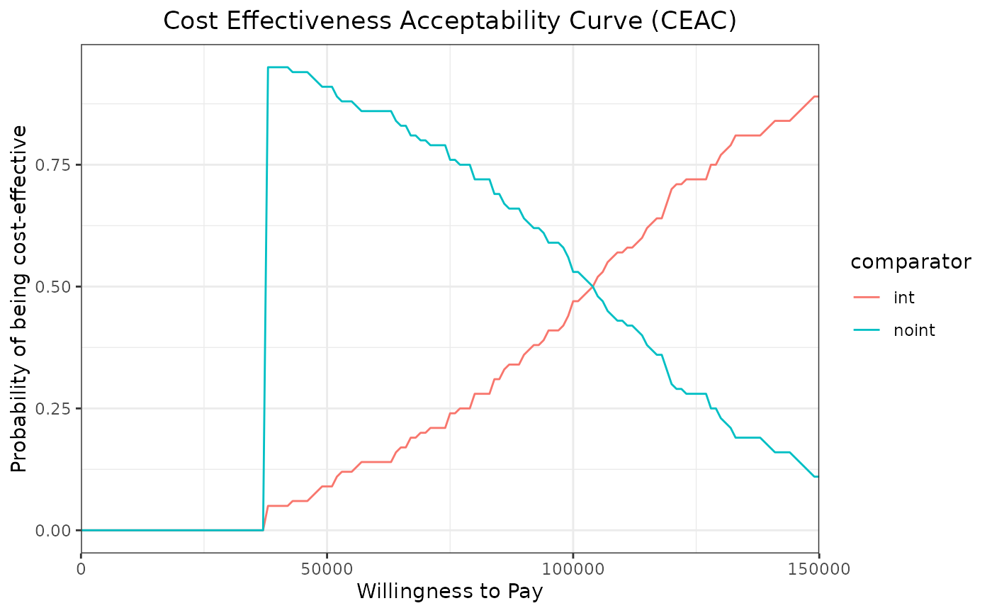
ceaf <- ceac_out %>%
  group_by(wtp) %>%
  mutate(max_prob=prob_best==max(prob_best)) %>%
  filter(max_prob==TRUE)

ggplot(ceaf,aes(x=wtp,y=prob_best,group=comparator,col=comparator)) +
  geom_line()+
  xlab("Willingness to Pay") +
  ylab("Probability of being cost-effective")+
  theme_bw() +
  scale_x_continuous(expand = c(0, 0)) +
  ggtitle("Cost Effectiveness Acceptability Frontier (CEAF)")+
  theme(plot.title = element_text(hjust = 0.5))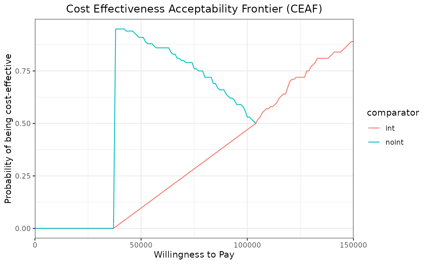
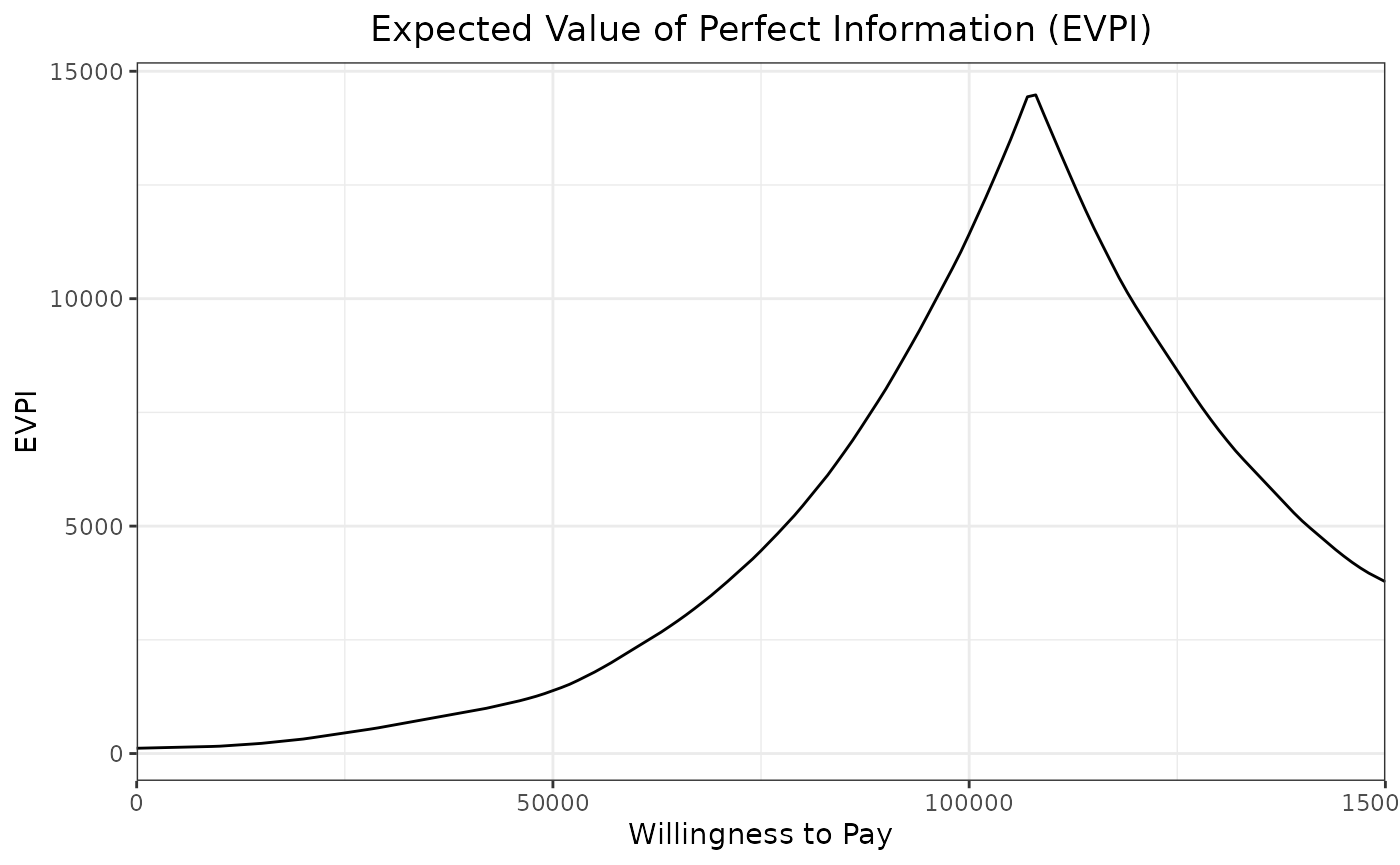
EVPI
Similarly to ceac_des, the function evpi_des also allows to compute the EVPI.
evpi_out <-evpi_des(wtp,results)

ggplot(evpi_out,aes(x=wtp,y=evpi)) +
  geom_line()+
  xlab("Willingness to Pay") +
  ylab("EVPI")+
  theme_bw() +
  scale_x_continuous(expand = c(0, 0)) +
  ggtitle("Expected Value of Perfect Information (EVPI)") +
  theme(plot.title = element_text(hjust = 0.5))