Mathematical Deep Dive

Definition and parameterization of Morlet wavelets

Background and setting

Despite the popularity and extensive use of Morlet wavelets for M/EEG analysis, differences in notation and parameterization used in the literature can be confusing. In the following, we provide visual and formal definitions, introduce our logarithmic parameterization, and establish its link with other parameterizations.

First of all, Morlet wavelets (Morlet et al. 1982) extend Gabor wavelets (Gabor 1946): Both, Gabor wavelets and Morlet wavelets are obtained by multiplying a complex sine-wave (oscillation) with a Gaussian taper. By construction, following from the uncertainty principle, Gabor and Morlet wavelets will also have a Gaussian shape in the frequency domain (if finite window lengths are neglected). Morlet wavelets define families of Gabor wavelets in which width and frequency are logarithmically scaled (Morlet et al. 1982; Tallon-Baudry et al. 1996). This means that a single Morlet wavelet is essentially a Gabor wavelet.

Gabor and Morlet Wavelets

To capture the variations of the spectral content of a signal over time, Gabor introduced in 1946 a basis of elementary waveforms, also known as time-frequency atoms (Gabor 1946). Such wavelets provide a localized time-frequency representation of the signal with an optimal tradeoff between time and frequency precision. Later, in 1982, Morlet adapted these wavelets to include a logarithmic scale in octave for the frequency of the sine wave and the width of the Gaussian window (Morlet et al. 1982). This scaling means that with increasing frequency, the wavelet becomes more time-localized (narrower time window) and less frequency-localized in (wider frequency bandwidth). Such wavelets, henceforth referred to as Morlet wavelets, account for log-frequency behavior and can be better suited for electrophysiological signals (Tallon-Baudry et al. 1996).

Essential design choice

A key feature of our parameterization is to express the Gaussian taper in terms of its spectral smoothing, i.e., spectral bandwidth (\(bw\)), logarithmically in units of octaves (Hipp et al. 2012).

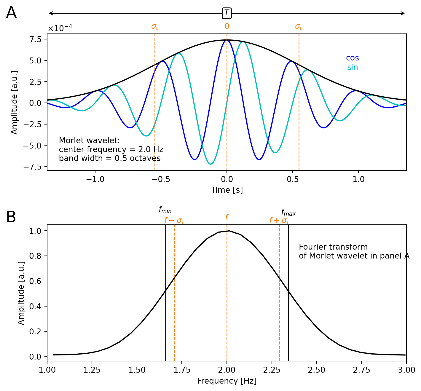
Let’s consider an example of a Morlet wavelet with a center frequency of interest \(f=2 Hz\) and a bandwidth of \(bw=0.5 oct\). The example Morlet wavelet is illustrated in Figure 1.

import numpy as np
import matplotlib.pyplot as plt
import matplotlib.transforms as transforms

# parameter
sfreq = 1000.
foi = 2.0
bw = 0.5

# for arithmetic mean
foi_min = 2 * foi / (2 ** bw + 1)
foi_max = 2 * foi / (2 ** -bw + 1)
df = foi_max - foi_min # frequency smoothing / FWHM
sf = df / (2*np.sqrt(2*np.log(2))) # map FWHM to sigma_f
st = 1 / 2 / np.pi /sf # sigma t (uncertainty relation)
kernel_width = 5
T = kernel_width * st
T = np.round(T * sfreq)  / sfreq
n_win = np.round(T * sfreq)
time = np.arange(-n_win / 2, n_win / 2) / sfreq
freq = np.arange(0, n_win) / T
Z = time / st
gaussian = np.exp(-(1 / 2) * Z ** 2)
gaussian /= np.sum(gaussian)
oscillation = np.exp(1j * 2 * np.pi * foi * time)
kernel = (gaussian * oscillation)

#freq = np.arange(0, len(kernel)) / T
freq_high_res = np.arange(0, 2**14) / (2**14 / sfreq)
kernel_fft = np.fft.fft(kernel, 2**14)

fig, (ax1, ax2) = plt.subplots(2, 1, figsize=(7.5, 7))

# Panel A
ax1.plot(time, kernel.real, 'b')
ax1.plot(time, kernel.imag,'c')
ax1.plot(time, gaussian,'k')
ax1.ticklabel_format(axis='y', style='sci',
                     scilimits=(0, 0), useMathText=True)

trans = transforms.blended_transform_factory(
    ax1.transData, ax1.transAxes)

trans2 = transforms.blended_transform_factory(
    ax2.transData, ax2.transAxes)

ax1.text(-0.1, 1.15, 'A',
          {'color': 'k', 'fontsize': 20},
         horizontalalignment='center',
         verticalalignment='center', transform=ax1.transAxes)
ax1.text(0.85, 0.82, 'cos', 
         {'color': 'b'},
         horizontalalignment='center',
         verticalalignment='center', transform=ax1.transAxes)
ax1.text(0.85, 0.75, 'sin', 
         {'color': 'c'},
         horizontalalignment='center',
         verticalalignment='center', transform=ax1.transAxes)
ax1.text(-0.03, 0.15, 
         """
         Morlet wavelet:
         center frequency = %.1f Hz
         band width = %.1f octaves
         """ % (foi,bw),
         horizontalalignment='left',
         verticalalignment='center', transform=ax1.transAxes
)

ax1.axvline(0, linewidth=1, linestyle='--', color='#ff7f0e')
ax1.axvline(-st, linewidth=1, linestyle='--', color='#ff7f0e')
ax1.axvline(st, linewidth=1, linestyle='--', color='#ff7f0e')

ax1.text(0.5, 1.05, r'$0$', horizontalalignment='center',
         verticalalignment='center', transform=ax1.transAxes, color='#ff7f0e')
ax1.text(-st, 1.05, r'$\sigma_t$', horizontalalignment='center',
         verticalalignment='center', transform=trans, color='#ff7f0e')
ax1.text(st, 1.05, r'$\sigma_t$', horizontalalignment='center',
         verticalalignment='center', transform=trans, color='#ff7f0e')

ax1.annotate("", xy=(-kernel_width/2*st, 1.15
), xytext=(kernel_width/2*st, 1.15),
             arrowprops=dict(arrowstyle="<->", connectionstyle="arc3"),
             xycoords=trans, textcoords=trans)
ax1.text(0.5, 1.15, r'$T$',
         {'color': 'black', 'fontsize': 10, 'ha': 'center', 'va': 'center',
          'bbox': dict(boxstyle="round", fc="white", ec="black", pad=0.2)},
         transform=ax1.transAxes
)

ax1.set_xlabel('Time [s]')
ax1.set_ylabel('Amplitude [a.u.]')
ax1.set_xlim(-T/2, T/2)

# Panel B
ax2.text(-0.1, 1.05, 'B',
          {'color': 'k', 'fontsize': 20},
         horizontalalignment='center',
         verticalalignment='center', transform=ax2.transAxes)

idx = (freq_high_res >= 1) & (freq_high_res <= 3)
ax2.plot(freq_high_res[idx], np.abs(kernel_fft[idx]), color='black')
ax2.set_xlabel('Frequency [Hz]')
ax2.set_ylabel('Amplitude [a.u.]')

ax2.axvline(foi, linewidth=1, linestyle='--', color='#ff7f0e')
ax2.axvline(foi-sf, linewidth=1, linestyle='--', color='#ff7f0e')
ax2.axvline(foi+sf, linewidth=1, linestyle='--', color='#ff7f0e')
ax2.text(0.5, 1.05, r'$f$', horizontalalignment='center',
         verticalalignment='center', transform=ax2.transAxes, color='#ff7f0e')
ax2.text(foi-sf, 1.03, r'$f-\sigma_f$', horizontalalignment='center',
         verticalalignment='center', transform=trans2, color='#ff7f0e')
ax2.text(foi+sf, 1.03, r'$f+\sigma_f$', horizontalalignment='center',
         verticalalignment='center', transform=trans2, color='#ff7f0e')

ax2.axvline(foi-df/2, color='black', linewidth=1)
ax2.axvline(foi+df/2, color='black', linewidth=1)
ax2.text(foi-df/2, 1.11, r'$f_{min}$', horizontalalignment='center',
         verticalalignment='center', transform=trans2, color='black')
ax2.text(foi+df/2, 1.09, r'$f_{max}$', horizontalalignment='center',
         verticalalignment='center', transform=trans2, color='black')

ax2.text(0.7, 0.8, 'Fourier transform\nof Morlet wavelet in panel A',
         {'color': 'k'},
         horizontalalignment='left',
         verticalalignment='center', transform=ax2.transAxes)

ax2.set_xlim(1, 3)

plt.tight_layout();

Figure 1: Example Morlet wavelet in time and frequency domain (a.u., arbitrary units).

Morlet wavelet parameterization

In our parameterization, we describe Morlet wavelets families by the spectral smoothing, i.e. spectral bandwidth (\(bw\)). In the following, we detail, how the Morlet wavelets are derived for center frequencies \(f\) .

A bandpass filter, that a Morlet wavelet basically is, is described by the two edge frequencies, \(f_{min}\) and \(f_{max}\), where the signal subjected to the filter is attenuated by 50% (see Figure 1 panel B). We define the bandwidth of the filter as:

\[ bw = log_2\left(\frac{f_{max}}{f_{min}}\right) \tag{1}\]

For a given center frequency \(f\) and a desired spectral bandwidth \(bw\), \(f_{min}\) and \(f_{max}\) can then be derived as follows:

Note

Auxiliary calculations \[ f = \frac{f_{min} + f_{max}}{2} \rightarrow f_{min} = 2f-f_{max} \]

\[ bw = log_2\left(\frac{f_{max}}{2f-f_{max}}\right) \]

\[ f_{min} = \frac{2f}{2^{bw} + 1} \tag{2}\]

\[ f_{max} = \frac{2f}{2^{-bw} + 1} \tag{3}\]

Note

Alternatively, one could use a geometric mean definition (implemented in our package but our default is the arithmetic mean)

\(f = \sqrt{f_{min}f_{max}} \rightarrow f_{max} = \frac{f^2}{f_{min}}\)

\(bw = log_2(\frac{f^2}{{f_{min}}^2}) = 2log_2(\frac{f}{f_{min}})\)

\(f_{min} = 2^{-bw/2}\)

\(f_{max} = 2^{bw/2}\)

Using the relationship between the standard deviation and the FWHM (full width at half maximum) for a normal distribution, we find:

\[ FWHM = f_{max}-f_{min} = 2\sqrt{2ln(2)}\sigma_f \tag{4}\]

\[ \sigma_f = \frac{f_{max}-f_{min}}{2\sqrt{2ln(2)}} \tag{5}\]

With the uncertainty principle we can derive \(\sigma_t\) \[ \sigma_t = \frac{1}{2\pi\sigma_f} = \frac{\sqrt{2ln(2)}}{\pi\left(\frac{2f}{2^{-bw} + 1}-\frac{2f}{2^{bw} + 1}\right)} \tag{6}\]

The Morlet wavelet for center frequency \(f\) and spectral smoothing \(bw\) is then (A is a normalization constant):

\[ W(t|f,\sigma_t(bw)) = A e^{-\left(\frac{t}{2\sigma_t}\right)^2}e^{i2\pi f t} \tag{7}\]

The convolution kernel that implements a Morlet wavelet has finite length. The length can be expressed in multiples of the temporal standard deviation of the Gaussian taper \(\sigma_t\). In our implementation this is the parameter kernel_width with the default value 5, corresponding to an extend of the Gaussian taper of \(\pm 2.5 \times \sigma_t\).

Selection of a grid of center frequencies for spectral analyses

Our Morlet wavelet package implements a grid with center frequencies spaced logarithmically according to the exponentiation of the base 2 with exponents ranging from \(f_{min}\) (e.g. 1 Hz, exponent 0) to \(f_{max}\) (e.g. 32 Hz, exponent 5) in steps \(delta\) (e.g. 1/8 oct). This ensures a coverage of frequencies that is coordinated with the spectral bandwidth and ensures a homogeneous coverage in the logarithmic frequency space.

Relationship between the bandwidth in octaves and the characteristic Morlet wavelet parameter \(q\)

A common way to parameterize Morlet wavelets is the characteristic parameter \(q\) (Tallon-Baudry et al. 1996; Oostenveld et al. 2011). See also, MNE-Python examples.

\[ q=f/\sigma_f \tag{8}\]

From Equation 6 and Equation 8 follows:

\[ q=\frac{\sqrt{2ln(2)} 2 f}{\left(\frac{2f}{2^{-bw} + 1}-\frac{2f}{2^{bw} + 1}\right)} \tag{9}\]

Note

Auxiliary calculation \[ \frac{2f}{2^{-bw} + 1}-\frac{2f}{2^{bw} + 1}=\frac{2f\left(2^{bw}-2^{-bw}\right)}{2^{bw}+2^{-bw}+2} \]

\[ q=\frac{2^{bw}+2^{-bw}+2}{2^{bw}-2^{-bw}} \sqrt{2ln(2)} \tag{10}\]

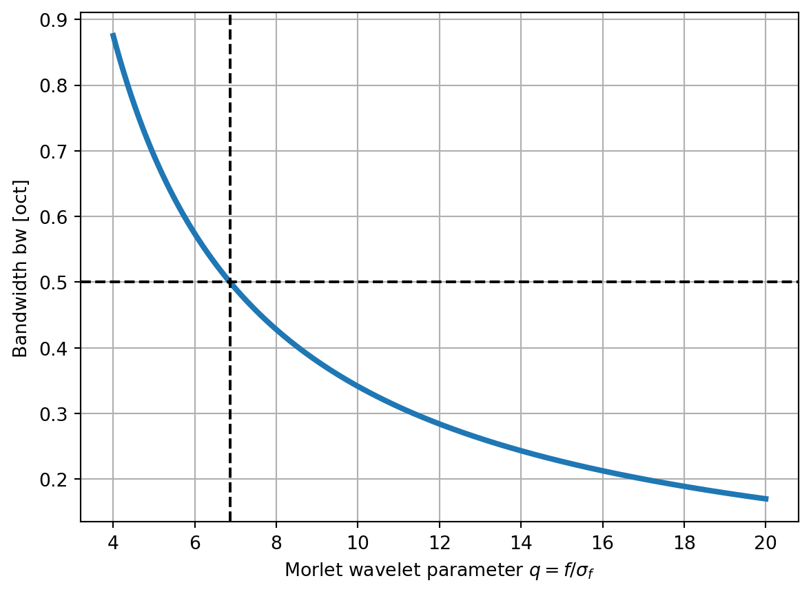
Applied, to our defaults of \(bw=0.5\), using the arithmetic mean, we find \(q=6.9\), which is close to the \(q=7\) that is used in literature (Tallon-Baudry et al. 1996).

def bw2q(bw):
    L = np.sqrt(2*np.log(2))
    return (2 ** bw + 2 ** - bw + 2) / (2 ** bw - 2 ** - bw) * L

bw = 0.5
q = bw2q(bw)
print(f"q(bw={bw:0.2f}) = {q:0.2f}")

q(bw=0.50) = 6.86

With this we can also compute the bandwidth \(bw\) from a given \(q\) by inverting Equation 10:

Note

Auxiliary calculations

\[ Def: \lambda=\sqrt{2 ln(2)} \]

\[ 2^{bw} \lambda + 2^{-bw} \lambda + 2 \lambda -q 2^{bw} + q 2^{-bw} = 0 \]

\[ 2^{bw}(\lambda - q)+2^{-bw}(\lambda + q) + 2\lambda=0 \]

\[ \left(2^{bw}\right)^2+\frac{\lambda+q}{\lambda-q}+2\frac{\lambda}{\lambda - q} 2^{bw}=0 \]

\[ \left(2^{bw}+\frac{\lambda}{\lambda-q}\right)^2=\frac{\lambda^2}{(\lambda - q)^2}-\frac{\lambda+q}{\lambda-q} \]

\[ bw = log_2\left( \pm\sqrt{\frac{\lambda^2}{(\lambda-q)^2}-\frac{\lambda+q}{\lambda-q}} - \frac{\lambda}{\lambda-q} \right) \tag{11}\]

def q2bw(q):
    L = np.sqrt(2*np.log(2))
    return np.log2(
        np.sqrt((L ** 2) / (L - q) ** 2 - (L + q) / (L - q)) - L / (L - q)
    )
q = 6.86
bw = q2bw(q)
print(f"bw(q={q:0.2f}) = {bw:0.2f}")

bw(q=6.86) = 0.50

This allows us to plot the following relationship between our bandwidth the the classical \(q\) parameter (see Figure 2).

q = np.linspace(4, 20, 1000)
bw = q2bw(q)
plt.plot(q, bw, linewidth=3)
plt.xlabel(r"Morlet wavelet parameter $q=f/\sigma_f$")
plt.ylabel("Bandwidth bw [oct]")
plt.axvline(bw2q(0.5), color='k', linestyle='--')
plt.axhline(0.5, color='k', linestyle='--')
plt.grid(True)

Figure 2: Relationship between characteristic Morlet-wavelet parameter and bandwidth in octaves. Black lines indicate the mapping from our default bandwidth to \(q\).

References

Gabor, Dennis. 1946. “Theory of Communication. Part 1: The Analysis of Information.” Journal of the Institution of Electrical Engineers-Part III: Radio and Communication Engineering 93 (26): 429–41.

Hipp, Joerg F, David J Hawellek, Maurizio Corbetta, Markus Siegel, and Andreas K Engel. 2012. “Large-Scale Cortical Correlation Structure of Spontaneous Oscillatory Activity.” Nature Neuroscience 15 (6): 884–90.

Morlet, J., G. Arens, E. Fourgeau, and D. Giard. 1982. “Wave Propagation and Sampling Theory—Part II: Sampling Theory and Complex Waves.” GEOPHYSICS 47 (2): 222–36. https://doi.org/10.1190/1.1441329.

Oostenveld, Robert, Pascal Fries, Eric Maris, and Jan-Mathijs Schoffelen. 2011. “FieldTrip: Open Source Software for Advanced Analysis of MEG, EEG, and Invasive Electrophysiological Data.” Computational Intelligence and Neuroscience 2011: 1–9.

Tallon-Baudry, Catherine, Olivier Bertrand, Claude Delpuech, and Jacques Pernier. 1996. “Stimulus Specificity of Phase-Locked and Non-Phase-Locked 40 Hz Visual Responses in Human.” Journal of Neuroscience 16 (13): 4240–49.