addpath('./matlab')MATLAB functionality
We perform the same computations using MATLAB.
With a few exceptions, the arguments are named the same.
The same default options are set.
The examples below processes the MNE sample EEG data in MATLAB and then computes power spectra as in the EEG power.
Note
For building this example, you need the Jupyter MATLAB proxy. To make it work, closely follow the GitHub. In particular, make sure your Python and Jupyter versions are compatible and MATLAB is properly added to your path. A good test is trying the Open MATLAB from within Jupyter Lab.
Moreover, we assume the MNE-MATLAB toolbox was added to the MATLAB path and the code is run from the root of the code repository.
Finally, we assume Python is installed with MNE onboard.
Loading the matlab functions.
fprintf('MATLAB version\n')
version
MATLAB versionans = '9.11.0.1809720 (R2021b) Update 1'
load MNE samlpe EEG data
[status, data_path] = system('python -c "import mne; print(mne.datasets.sample.data_path(), end=str())"')status = 0
data_path = '/Users/engemand/mne_data/MNE-sample-data'
fname = strcat(data_path, '/MEG', '/sample', '/sample_audvis_raw.fif');raw = fiff_setup_read_raw(fname);Opening raw data file /Users/engemand/mne_data/MNE-sample-data/MEG/sample/sample_audvis_raw.fif...
Read a total of 3 projection items:
PCA-v1 (1 x 10²) idle
PCA-v2 (1 x 10²) idle
PCA-v3 (1 x 10²) idle
Range : 25800 ... 192599 = 42.956 ... 320.670 secs
Ready.picks_eeg = fiff_pick_types(raw.info, 0, 1);
picks_eeg(53) = []; % flat channel EEG 53[data, times] = fiff_read_raw_segment(raw, raw.first_samp, raw.last_samp, picks_eeg);Reading 25800 ... 192599 = 42.956 ... 320.670 secs... [done]data = data - mean(data, 1); %average ref for comparability with Python exampleplot(data(1:10,1:3000)' * 1e6)
set(gcf, 'Units', 'inches');
screenPosition = get(gcf, 'Position');
set(gcf, 'Position', [screenPosition(1), screenPosition(2), 8, 4]);
ylabel('EEG [${\mu V}$]', 'Interpreter','latex')
xlabel('Time [ms]')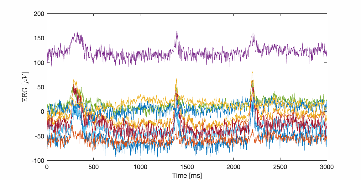
Compute power from Morlet Wavelets
help("ro_freq_meeglet") meeglet (ver 1.0)
Denis Engemann & Jörg Hipp, Feb 2024
Log-spaced frequency transform using Morlet wavelets for continous
electrophysiological signals. Derive power, covariance and various
conncetivity metrics
% Input
- dat ... [channels x samples], set invalid data sections to NaN;
Input signal needs to have in µV
- cfg ... struct, see script itself for default parameters, cfg.fsample
has to be set by the user
% Output
Metrics indicated in cfg.output (default: all)
Values returned as fields in struct out:
- foi .. frequencies for which below metrics are derived in Hz
- n .. number of time-windows used to compute below metrics
- cfg .. the cfg struct containing all parameters
- unit .. unit of the power spectral density (pow)
- pow .. Power spectrum. The total power in µV² for a channel (ich) over
the frequency range [cfg.f_start,cfg.f_end] can be derived as:
if cfg.density is 'linear' -> total_power = trapz(foi,pow(ich,:))
if cfg.density is 'log2' (default) -> total_power = trapz(log2(foi),pow(ich,:))
- csd .. Cross-spectral density matrix
- cov .. Covariance matrix, same as real(csd)
- coh .. Coherence, compley values use coh.*conj(coh) to derive magnitude squared coherence
- icoh .. Imaginary coherence (Nolte et al., Clin Neurophys, 2004);
function returns signed values, use abs(icoh) to be line with the original definition
is the same as the cross-sepectral density of the orthogonalized signal
- plv .. Phase-locking value (Lachaux et al., HBM, 1999)
- pli .. Phase lag index (Stam et al., HBM, 2007); function returns signed values,
use abs(pli) to be in line with the original definition;
is the same as the phase-locking value of the orthognalized signal.
- dwpli .. Debiased weighted phase lag index (Vinck et al., NeuroImage 2011)
- r_plain .. Power correlation
- r_orth .. Orthogonalized power correlation (Hipp et al., Nature Neurosci, 2012)
- gim .. Global interaction measure (Ewald et al., NeuroImage, 2012)
%% Example 1:
% Single channel with background noise and sine wave at 10 Hz
fsample = 250;
T = 60; % [s]
n_chan=1;
n_sample = T*fsample;
t=(0:n_sample-1)/fsample; % [s]
f = 10; % Hz
rng(0)
x=randn(n_chan,n_sample)*10+repmat(sin(2*pi*f*t)*10,[n_chan,1]); % [µV]
%
clear cfg
cfg.fsample = fsample;
cfg.delta_oct = 0.05;
cfg.foi_start = 0.1; % given parameterization cannot start at 0
cfg.foi_end = fsample/2;
cfg.density='Hz';
% µV²/Hz density
freq = ro_freq_meeglet(x,cfg);
figure('Color','w')
plot(freq.foi,freq.pow,'r')
xlabel('Frequency (Hz)'), ylabel(sprintf('%s',freq.unit))
% µV²/oct density
cfg.density='oct';
freq2 = ro_freq_meeglet(x,cfg);
%
% Test Parseval's theoreme, i.e. power should be identical in time and
% frequency domain (note: expected not to numerically match given the parameterization)
Pt = mean(x.^2,2); % time domain; same as sum(x.^2*dt)/T, where dt=1/fsample, T=n_sample*dt
Pf_lin = sum(freq.pow(1:end-1).*diff(freq.foi)); % Frequency domain with linear frequency spaceing
Pf_log = sum(freq2.pow(1:end-1).*diff(log2(freq2.foi))); % Frequency domain with log frequency spaceing
fprintf('Power derived in time and frequency domains:\nPt = %.1f µV²\nPf_lin = %.1f µV²\nPf_log = %.1f µV²\n',Pt,Pf_lin,Pf_log)
%% Example 2:
% Artificial signal with background noise on 19 channels and two coherent sine-waves at two channels
fsample = 250; % [Hz]
T = 60; % [s]
n_chan = 19;
n_sample = T*fsample;
t=(0:n_sample-1)/fsample; % [s]
f = 10; % [Hz]
rng(0)
x=cumsum(randn(n_chan,n_sample),2); x=5*x./repmat(std(x,[],2),[1,size(x,2)]); % pink noise
x(1,:) = x(1,:)+sin(2*pi*f*t);
x(10,:) = x(10,:)+sin(2*pi*f*t+pi/4);
%
clear cfg
cfg.output={'pow','coh','icoh'};
cfg.fsample = fsample;
freq = ro_freq_meeglet(x,cfg);
%
figure('Color','w')
h=subplot(2,1,1); plot(log2(freq.foi),mean(freq.pow)), set(h,'XTick',log2(freq.foi(mod(log2(freq.foi),1)==0)),'XTickLabel',freq.foi(mod(log2(freq.foi),1)==0))
title('Power spetral density'), xlabel('Frequency [Hz]'), ylabel(freq.unit), a=axis; a(3)=0; axis(a)
subplot(2,2,3), imagesc(abs(freq.coh(:,:,20)),[0,1]), axis square, colorbar, title(sprintf('abs(COH), f=%.1fHz',freq.foi(20)))
subplot(2,2,4), imagesc(freq.icoh(:,:,20),[-1,1]), axis square, colorbar, title(sprintf('iCOH, f=%.1fHz',freq.foi(20)))
cfg.fsample = raw.info.sfreq;
cfg.output = {'pow'}
cfg = struct with fields:
fsample: 600.6150
output: {'pow'}
out = ro_freq_meeglet(data * 1e6,cfg);Morlet wavelet transform [.................................] 8.1 secoutout = struct with fields:
cfg: [1x1 struct]
foi: [2 2.1810 2.3784 2.5937 2.8284 3.0844 3.3636 3.6680 4 4.3620 4.7568 5.1874 5.6569 6.1688 6.7272 7.3360 8 8.7241 9.5137 10.3747 11.3137 12.3377 13.4543 14.6721 16 17.4481 19.0273 20.7494 22.6274 24.6754 26.9087 29.3441 32]
pow: [59x33 double]
pow_var: [59x33 double]
unit: 'µV²/oct'
pow_median: [59x33 double]
pow_geo: [59x33 double]
n: [402 439 479 523 570 621 677 741 806 879 961 1046 1139 1241 1353 1473 1616 1752 1914 2082 2281 2486 2687 2923 3204 3472 3787 4167 4505 4902 5377 5748 6412]
qt: 6.8624
bw_oct: 0.5000
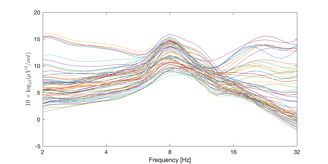
Plot log power and on log frequency grid
log_foi = log2(out.foi);
log_pow_db = 10 * log10(out.pow);plot(log_foi, log_pow_db')
xlabel('Frequency [Hz]')
xticks([1, 2, 3, 4, 5]);
xticklabels([2, 4, 8, 16, 32]);
ylabel('${10 \times \log_{10}(\mu V ^ 2 / oct)}$','Interpreter','Latex')
set(gcf, 'Units', 'inches');
screenPosition = get(gcf, 'Position');
set(gcf, 'Position', [screenPosition(1), screenPosition(2), 8, 4]);